Hi, everyone. Thank you DFRWS for having me, and thank you for your interest in this short presentation. These are observations from a little side quest that I had to do within my PhD. Here, let me take away the title and show you the clear version of my background.
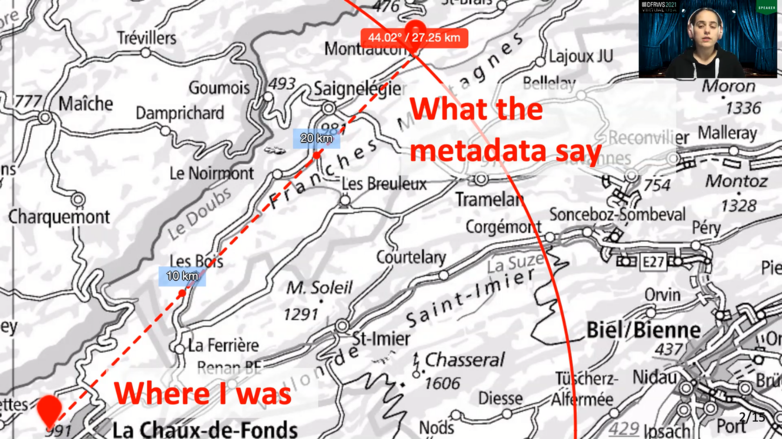
The story behind this map is me taking a picture near a city in the canton of Neuchâtel in Switzerland. And it being located in another canton, nowhere near where I was in reality. As illustrated here, the horizontal error between the two places is approximately around 27 kilometer. It is the most extreme value that was gathered in this exploratory study, and it sums up all the questions that I had about interpreting and communicating digital forensic issued information, and especially in this case, about how to understand the value of the geolocation metadata of a picture taken with a mobile phone.
So normally my main subject of study is uncertainty in digital forensic science. The first questions were around the communication of results by forensic expert and how the information carried by digital traces were being used in the judicial process. Being interested in communicating the value of the information carried by a digital trace, we quickly were interested in sources of uncertainty and what kind of parameters could influence the information carried by the trace. Does uncertainty exist? Can we observe it? Can we define influencing factors? We had to make some IRL observations to try and match a theoretical model with reality. And here we were, with a new side quest: geolocation.
But before geolocation and all that, a little bit of theory. By breaking down the trace in accordance to its definition, the influencing factors were divided into four different axes: time, carrier, activity, and source. The time extends from the generation of the trace until its disappearance, and includes the possibility of detection and observation as pivotal points of its existence.
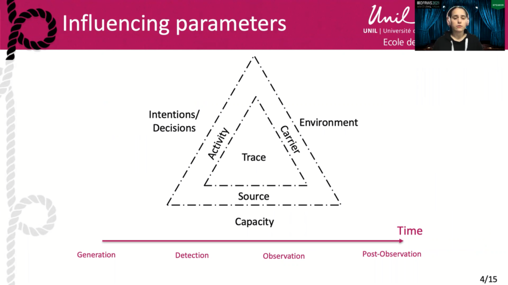
The carrier is what carries information. It is both understood in and influenced by its environment, which can be material or virtual. The source is at the origin of the action, and therefore the traces generated. Regarding traces linked to a computer system, it can be assumed in particular that the hardware and software used during the events may have an influence on the traces taken during the investigation. For instance, the computer skills of the author or the action and his abilities when using them are among the variables that can influence the state of the source during the action.
By developing Locard’s postulate, the trace only exists following the presence or absence of an event. With the exception of extreme cases, it is generally accepted that the trace is a consequence of the presence or absence of activity. Therefore, we can assume that variations in activity will be reflected in the traces generated. In this model, it has been intentionally put forward that variations in an activity can in particular depend on human intentions. This highlighting allows for an easier application afterwards to our side quest.
So back to it, now. Applying this model of source to the geolocation of a mobile phone, here are the different influencing parameters that were identified. On the activity side, you might need to consider the mobility of the device, the tampering of traces, and general user usage. Was the phone moving or not? What speed? Was there tempering? Obfuscation? Was the phone just turned on right before taking the picture?
On the carrier side, the environment might be of importance. How was configured the phone to save the data you will be analyzing? Did it have access to network coverage? Which applications were installed on the phone? Do they have access to the information that was saved on this phone?
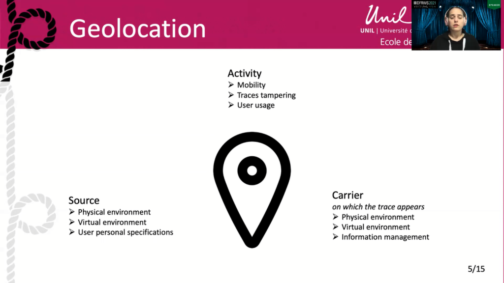
And finally on the source side. We weren’t focusing on this in this exploratory study, as otherwise the amount of variables would have exploded. The environment, be it physical or virtual, would be especially important when creating geolocation metadata. Which network is available? Which model of phone is being used? What it’s GNSS chipset? What is the environment where you’re taking your picture? If the wifi is being used? How is built the database? How can you access it? Which search algorithm is being used?
Those are a small subset of all possible variables, and without even taking into consideration the user personal specification. What are his preferences? Which manipulations were done on his phone? In this study, we tried to remove a maximum amount of variables by using two similar phones, always following the same path, taking pictures at the same place and transporting the phone from one place to another in the same way.
So here you can see that three paths were followed, always in the same direction as I said before, and with approximately the same walking speed between the different points to be photographed. I had two phones within my jacket. So two phones had the same hardware and software configuration to limit variables. The standard one was always connected to 4G and had the possibility to locate itself using GNSS and wifi. The other one (the experimental one) didn’t have those possibilities and was limited in its connection to the cellular network. For one third of the data gathering, it would be connected to 2G, 1 third to 3G, and the last third to 4G.
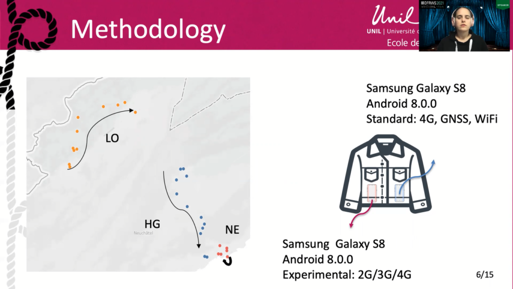
In the end, each route was travelled at least nine times, only one picture being taken by location by phone per day. Some days had to be repeated due to technical problems. This happened between November and March. The first route was in a rural area with a long passage near a border through fields and forests. The second path was at a lower altitude in a rural area with fields, forests and [inaudible].
Halfway through, a measuring point was in the middle of a village. Finally, the last one was in urban area, in the city of Neuchâtel, with a point on the edge of Lake Neuchâtel. These different routes made it possible to vary the external environment, as well as the quality of some network and/or the satellite reception. In total 497 pictures were gathered in 29 places.
So here’s the results. Here you can see the distribution of all data. There are multiple information that can be gathered from this plot. First, some data points have an horizontal error higher than 20,000 meters. Then the distribution is highly skewed to the left, which indicates there’s those extreme data (here at 10,000 meters and here 20,000 meters) might be outliers as the majority of the population is on the far left of the plot.
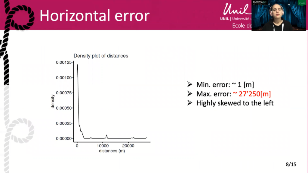
The distribution doesn’t seem normal, and we will want to take that into consideration when we will test our hypothesis. We also might want to remove the outliers to see its effects on our distribution. As you can also see, the minimal horizontal error is at 1 meter and the maximum at 20,250 meters. So the distribution is quite wide.
While looking more closely at the collected data, it appeared really quickly that quite a big amount of pictures didn’t have any geolocation metadata. The experimental phone had 53 pictures without any geolocation metadata, and the standard phone, with GNSS positioning available, had 96 of them without any geolocation information. This was particular to some places with, for example, two of them having only 20% of their pictures with geolocation metadata.
After confirming that the two distribution, one per phone, were not normal, we used a Mann-Whitney test to check if the difference of horizontal error between the two distributions was significant, and it confirmed that indeed. The test was done on data collected with the 4G on, so it seems that this difference might come from the presence or absence of GNSS and wifi connections. Here you can see for yourself the difference of horizontal error on this box plot.
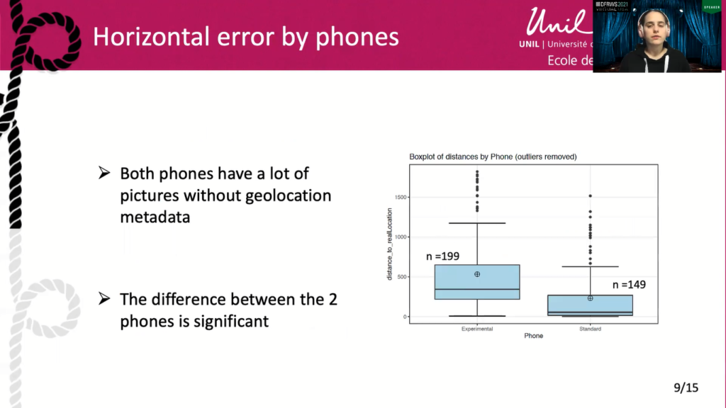
Regarding the whole distribution, it was decided to fix the outlier limit at 1,800 meter, as a majority of the data points were below this line. This means that in general, regardless of the phone or the place, most horizontal error fell below 2 kilometers. However, as we can see on this box plot, there seems to be some specific places gathering most of the outliers.
Regardless of the phone, four places make for 80% of the 34 outliers. We can also see on this plot that some places seems to have a higher variance regarding the horizontal error of the geolocation. This has led us to divide places into two groups, one with a lower variance, and one with more variability. In this last group, some data were really extreme and categorized as anomalies.
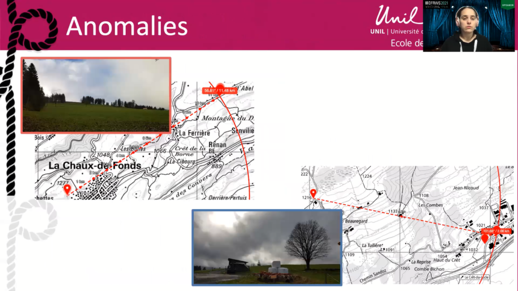
As said, right now, some of the outliers were really impressive and seemed to be difficult to explain. Even with the localization with GNSS activated, horizontal errors beyond 10 kilometers were formed for a place situated right at the border of a forest (the first example here) and of 2 kilometer for a place with an open sky and no visible obstacle, so the example is below.
With no GNSS activated, the horizontal error jumps to 20 kilometer and more for those two places, and more places have outliers. One outlier in particular is quite peculiar. The place is in the middle of the fields with an horizontal error, usually between 300 meters and 1,300 meter. And this outlier is located five kilometers away from the place. This goes in the direction of the value of the information from geolocation metadata being difficult to interpret.
Aside from the horizontal error, the directional error of the metadata can be calculated. The data here is coming from the phone with GNSS and wifi access. As previously said, some places have few data points. It is visible here as the length of the box is relative to the numbers of pictures taken with geolocation metadata.
The picture are also distributed within one of the 16 directions of the windrose (north is up). As we can see here, the directional arrow seems to really differ from one place to another. About half of them (the red ones) have a strong inclination to a particular direction. The other half seems to be more equally distributed, and I have some example to illustrate all that.
So here are two specific example of a directional error, not evenly distributed. The first picture illustrate the data collection at the port of Neuchâtel. The pictures were all taken at the most extreme point of the pier, and here we can see that the directional error is concentrated towards the city and the north.
Another example, this time again in Neuchâtel, but at the top of the stairs leading to the castle, as you can see from the picture. It is surrounded by high walls. The directional error here is oriented toward north-east, which is not the way down or up the path.
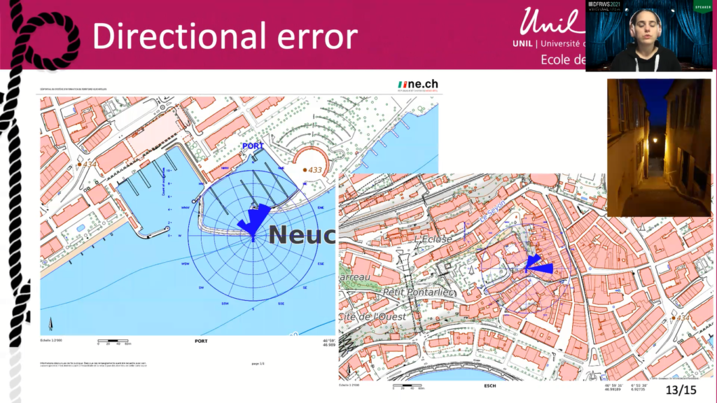
On the opposite, here are two example of a diversified error. The first one is on the front porch of a small church inside Neuchâtel. It is surrounded by buildings with one or two floors. We can see that the directional error goes in two very different directions. The reason, as before, is difficult to understand.
The last example is in the middle of the fields. Here, nothing obstruct the view in a parameter higher than 100 meter. The directional error seems evenly distributed. It is difficult to pinpoint a reason for these different behaviors, even more so that the data set is limited. More research would be needed to see if a pattern can be observed.
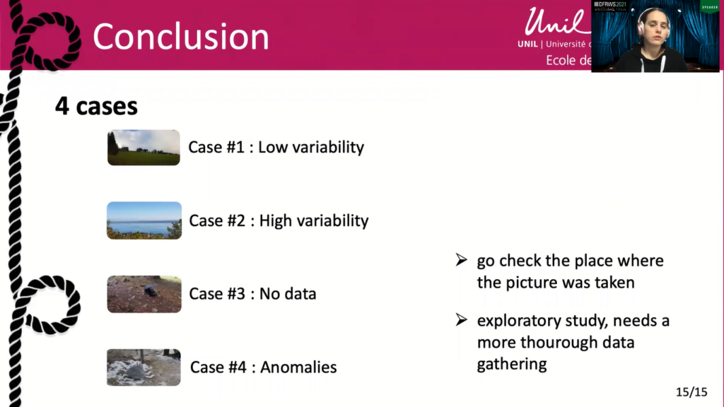
To conclude, four types of location seems to have been identified in this exploratory study. In the first type of location, analysis of the pictures taken during the experiment showed little variability in the location of the picture, and the horizontal error was smaller than 2000 meter. It is possible in this kind of scenario, knowing that the phone used to take the picture was connected to 4G at time T, to quantify the probability that the picture was within a radius of X meter around the place visible in the picture.
Based on additional contextual data, final categories can be drawn. For example, if we know that the device also has a satellite location and its wifi activated, the probabilities will vary depending on the proposition.
In the second case, a high variability was detected in the localization of the picture. In these cases, it will be much more difficult to assess the value of the information contained in the metadata based on propositions. It was difficult to pinpoint an explanation regarding the high variability in the accuracy of the localization.
In the third case, no geolocation information was found in the pictures taken during the experiment. Being able to say that at some location, you have more chances to not have geolocation data on the picture is really interesting. This information allows for an assessment of investigative eye practices, such as does the lack of geolocation data confirm the possibility that the person who took the picture didn’t want to be located, or is this phenomenon coming from the location?
Finally in the last type of location, the locations tested resulted in outliers and the value of the information can be estimated to be very low, regardless of the apparatuses under which it is examined. Errors ranging from 5 to 27 kilometers were spotted during the experiment without being able to identify any particular reason, which led us to the hypothesis that it is really difficult to identify problematic location without actually generating some geolocation data.
All this information can help a forensic expert in evaluating the trace in front of him, or the investigator, in deciding whether or not he should act upon the information reported to him.
Thank you for listening to me and thank you to the team at the University of Lausanne for helping me during this research. If you have any question, please, you can ask them now I will be happy to answer, or you can contact me on my email address or via Twitter. Thank you.


