Frank: Warm welcome also from my side. This is a presentation or some work that I did together with Peter. He reached out to me. He is in the States and he reached out and said, “hey, I saw online you the similarity guy. And I have some work here and you wanna collaborate on this?”
And I said, “oh, sure. Send it over.” And then we started a SMARC…I forgot the expression that he used, but you sprinkle some (I forgot the exact terminology that he used) but you sprinkle some more scientific stuff on it, and then it turns into a paper.
So, it was a really more practitioner driven in the beginning. He had a problem that he had to solve and I said, “hey, this is actually really interesting. Why not share this with the community?” And so it’s not similarity hashing, so that’s a big surprise! I’m here and not talking about that. I’m talking about something that is quite similar to it.
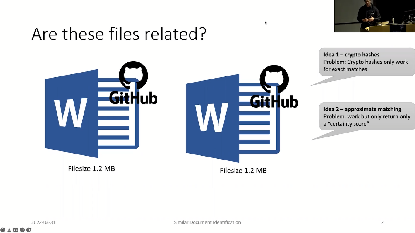
And so the question that we raised in the beginning was: are two files related. And the possibilities that we have is on the one hand we can say…or we can use the cryptographic hashes, but those will only identify complete identical files. So, that’s fast, efficient, but only identical files. And we’re not only talking…well, we’ll come back to this later.
Then the second question: okay, can we use approximate matching for our problem? And the problem with approximate matching is, for those of you who are familiar with it, you only get a certainty score. So, you only get a value saying, “yep, I’m confident that they are related”, but you don’t really know what it means, so it’s not defined.
And then we said, “okay, can we use something like the Levenshtein distance, for example?” So, for those not familiar with the Levenshtein distance, it’s a precise measure to measure the similarities/dissimilarity between two strings. So, it’s the…given the pair strings, it’s the number of single character edits to convert one into the other string, right? So, you can use inserts, deletes and substitutions, and to convert one string into the other.
So from AAA to BBB, there’s just 3. You have to delete all A’s and then…or replace…substitute all A’s by BS. And in the second example, it’s 2, because you can simply replace the F…uh, the B with an F and the one E with an R…A to convert them. So, then we said, “okay, that actually solves the problem that we have. So we wanna have a measure that gives us a score that means something to us, right? That we can…that is defined.”
And then, this is why I put like the file size up there, we then realized there is one problem is the run time with this approach. So, the problem is that it has a complex runtime making it fairly slow. And to give you an example, if you have two strings with about 50,000 characters and you do a comparison, I did it on my laptop, it was about 3.5 seconds. And 50,000 characters is not that much.
So this document, or if you talk about websites, like larger websites, or GitHub repositories, when you wanna compare source code, you have easily larger files. So, at this 1.2 megabyte file that we put up there as an example, it would be about 1.2 million characters.
So, it is impractically slow, at least on a regular hardware. So, it’s not feasible. There are some optimizations, so for those of you really deep into this material, yeah, you can optimize a little bit to get around this problem, but you can never reach the speeds that we reach with our estimation.
So, what is then the contribution? So, we developed a tool or a heuristic to estimate the Levenshtein distance of text pairs over a size range, many hundreds of times larger/faster than it is practical for calculating the exact value. And you can adjust the performance, so slash the settings by using parameters, and we have a GoLang implementation that is available. We also have Python and Java, and those would be available for those who are more familiar with those programming languages.
Why do we have three? He started in Java. I don’t like Java. Then I did it in Python, realized it’s super slow, and then I decided, okay, I’ll do it in GoLang again. And then I got really happy, because I now really like GoLang, but it’s a completely different story. Happy to share it later!
So, what is this algorithm about? We do estimate the Levenshtein distance in three steps, or we do a comparison in three steps.
The first step is we compress each document into a signature using a Loosy compression algorithm, LCA. This outputs pretty much just a randomly looking shorter text, and this is an example here on the…can I?…it just looks like randomly. It is based on an alphabet that we define.
And if we have these signatures, we then can, or we apply the original Levenshtein distance. So we shorten, we shrink the text in a particular way and use that downsized text and apply it in the original Levenshtein distance giving us some score. And then we do some back scaling, right? So we have then the Levenshtein distance on this compressed material, and then we have to scale it back roughly by the compression rate. It’s a little bit more complex, but that’s the idea.
So, when we then looked into this Lossy compression algorithm, what are the desired properties that we wanna have? So we need compression, of course. We don’t care if information gets lost because we don’t wanna have the original documents anyway. It needs to be deterministic.
So, if you, for example, use zip and you zip the same file twice and you gonna rate the hash value, there will be different, right? It’s not a deterministic algorithm. You wanna have runtime efficiency, so it needs to be like really fast that it’s worth it, and we wanted to have concatenation, what you would expect like in the real world, so if you have two hash values, you can concatenate them together and it’s pretty much like the same if you compare it or over the whole file. We achieved all of that.
For the last one, we settled with something that we simply say is good enough. So, it’s not perfectly there, but very close to it, to the concatenation property.
And then we use three parameters that adjust, or that allow us to configure our implementation. So, we have the compression rate, we have a neighborhood and we have the alphabet. The alphabet is simply our output, so the characters that we can use and there simply: larger is better.
So, the more characters we use, the more distribution we have and we can…it pretty much…but it’s hard to explain. It took me like, I think about a page, to describe these three parameters in the paper, so I’ll try best to keep it rather short here.
The compression rate is simply how much you wanna condense it. And there’s different scenarios, this is why we wanted to have this as a parameter. If you have very, very large files, you might have a larger compression ratio. You might have very small files there, you have like a very minimum one. And we use a neighborhood, this is pretty much kind of a sensitivity, how sensitive our algorithm will react to actual changes.
So, how does this procedure then work? We have a string and I have a better example, I think on the next slide. We define the digest, that’s simply like an empty string. We iterate through that string, so we have…we iterate through it based on the neighborhood size, so it’s pretty much like a kind of a window that goes through and compute a hash value.
So, here in this step 3. For this hash, we tried various implementations and then settled with Rabin-Karb because it’s simply very, very efficient and does exactly what we want to do. We store this result in T, do a simple modulor operation, and this is where this compression rate comes in.
I mean, people familiar with modulor, if you have like 100, 1000, this is how often it matches. And this way every time we hit a certain value, doesn’t matter which values it is here, 0 was simply the easiest. Then we would use our alphabet to choose one character out of this alphabet and add it to our signature. And then we continue with the next one.
So how does this look? So if we have like this particular string here, rather short string, and our parameters are set up here. The first iteration we have our neighborhood, which is 7 here, we would compute the hash value over that string at position 0 and do a modulor computation. This would be for example, here 59. And this is “T mod C unequal 0”, so we simply continue.
We now focus on this particular substring, so we move by pretty much one position and then do the same procedure pretty much, and we receive an 8, so we’ll also continue. And then here we receive like finally a 0.
And in this particular case, we go to our alphabet and choose pretty much out of our alphabet one character that will replace that string here from “LLO_WOR”, this string, or this particular substring, will be replaced with one character out of our alphabet that we defined. This is why a larger one, we have like more variety and makes it, like, stronger algorithm.
And these first characters…so first of all, those are simply replaced by one character, that’s already cutting it down. And these first two are completely ignored, right? So they will be completely ignored. And then we continue. So, here we would then add to our signature, the A and then simply continue and do this.
And this is why the neighborhood, for example, if you have a large neighborhood, then single swaps here impact a lot of neighborhoods. This is why there’s the sensitivity.
So, you would do this for the whole file. And depending on the compression rate that you set, you would reduce your algorithm and would get a signature, for example, that looks like text or like random text. Those familiar with ssdeep, it is pretty much similar to rolling hash that ssdeep uses.
So, we then generate like these eLD signatures that are comprised of a header and the actual digest. And the header is necessary to keep track of the parameters. Of course, we can only compare signatures that have the same settings. And what is mandatory here is the file length, as well as the digest.
The file length is needed for the scaling part, so we need to know what we actually condensed or what we worked on to reduce it. The others are somewhat optional. So, the file name is always helpful, that’s why we keep it. C and N, if you always use the same, you can, of course, you could remove that. But for simplicity we simply include this.
And then as I said, then we compare these signatures that we then have here using the regular Levinshtein distance. And once we have then the value, of course, this is many times smaller than the original version, what we then have to do is the back scaling.
And I particularly say here, it’s the unscientific description as we simply multiply with a compression rate. This is a little bit more complex so I put it down here, but we actually have to do, so we have to have some kind of very simplistic math to do here, but it’s not a single multiplication.
And the three considerations here is that the documents that have roughly the same size are, will have roughly the same size signature. This in return means if there’s a large difference in size, they will have also a different in length, and this different in length is already the minimum distance that they will have.
And then the last point unrelated documents usually have a Levinshtein distance that is shorter than their length. This means if you take two English texts, there is…and they both have a 100,000 characters, the Levenshtein distance will not be a 100,000, because every text contains, like, Es. So you can do it more efficient than using 100,000 substitution to go from one text to the other text.
And then when I read this and I was like, that’s interesting, but does this actually work? And then we did some testing and I was really surprised how good it works. The scenarios where it doesn’t work very well, I’ll come to those in scenarios where it actually works nicely.
So, the signature generation (before we talk about the evaluation), the signature generation: the run time is impacted by the hash function. So, because every string has to be processed, so we need an efficient hash function and the neighborhood because the neighborhood is what is hashed. The compression rate doesn’t matter here. So, the compression rate doesn’t impact that.
On the other hand, the signature comparison time, that is strongly influenced by the compression ratio. So, the more I compress, the shorter my signatures get and since the signatures are compared with the Levinshtein distance, the shorter, the better. So the shorter, the faster. And does not have an impact here. The precision is impacted by everything. So, the C, N, there’s some other parameters there that I’m not even gonna mention here.
And so we did some testing and this is all based on the GoLang implementation. So, what we did here is just to play around a little bit, to see the impact. And we used a constant C, and then various neighborhoods, and for Rabin-Karb, it doesn’t even matter so much, for other algorithms here it’s a little bit more significant.
So, this is why we then after seeing this we decided, okay, we’re gonna just stick to Rabin-Karb. This was a dataset about 7.2 GB, and we needed like 40 seconds to generate the signatures out of the 18,000 files and 7.2 GB. It is not exactly, so this is why the star is marked here. So I used for MD5 and FNV I was…didn’t wanna implement it on my own, so I used libraries, we had some casting to do. So this might have slowed down a little bit. If you natively implement it, then you might get a little bit faster.
Then for the signature generation part, we did comparisons and here we can see the more we shrink, the faster it gets, is pretty much the conclusion from this slide. And we did this on a smaller set. So we didn’t compare against all from the 18,000, but used a smaller set to give us an idea.
This is probably the most interesting table. That was like the part where we did then some testing, how can we find files? And this was done manually. And this is definitely an area of future work where we have to do more work. We had a file, we cloned the file and did manual operations.
And the center column here of the operation, this is describing what we did. So we deleted 10 lines, we deleted 10 lines at a different position. We deleted 52 lines at the beginning, 101 lines. This was just literally random things that I did. We deleted 7 chunks and so little bit larger paragraphs. 3 large chunks, 15 times 3 lines. So just to have some random operations to see how it works.
And we realized that it works well for deletions but problems with when they are spread out. So, we can see here, we have here the original Levinshtein distance, and here’s our estimations. So, we can see that sometimes even we have exact matches.
So, overall for this first batch, like rows 1-13, it works fairly nicely. Random inserts…the insert of the random A can cause a problem if there are too many, right? So, if there are small changes spread out, because we reduce it, we hash it, this is how this impacts it. Swapping was okay.
And of course the major problem is with many small changes throughout. So, what we did was one time we replaced all Bs (like the lowercase Bs), which was a 338 and then all Es, which are 3000 in this particular document, and then the numbers are significantly different.
So, if you look here, the original Levenshtein distance is exactly like 3080, that’s what you expect if you do this replacement. And here, our numbers are not as great anymore.
So how does it compare overall? We did then some more comprehensive…some additional tests to see how…so this was like a 20 comparisons here, so here we did like a little bit more testing, I think about like 200 and automatically evaluated than the results.
And we can say that overall the results were okay. This is at least how we would treat it and especially given the time. So for the original Levinshtein distance, we had to wait almost 10 minutes (or 9 minutes), and then with the C value of 11, we already brought this down to 3.5 seconds. And so it gets like significantly faster. And then for C, like 200, was like 0.3 seconds.
As I said, there’s a little bit more involved. So, the paper explains a little bit more about these parameters. For example, there is something an R value, which is the expected overlap per text. So, unfortunately this algorithm doesn’t easily…so you have to train this algorithm to perform.
So it is currently trained on English text. So, the R value that we have is for English text, and if you use another language where you have this different distribution of characters, for example, it will not as well perform. So, we have one particular script that does like the adjustment of the parameters that would have to run in order to get this expected overlap value, or the R value.
So, the algorithm could output a Levinshtein distance of 0, although there are minor differences. It will never do the other way around. So, we’ll never say bigger than 0, if strings are identical, right? So, this is like one of the trade ups that we have here. And it does not work well for short texts, but there we can simply, if they’re too short, we can fall back to the original Levenshtein distance. So that’s not really a problem.
How could this be used then? Because we only get, like, a distance measure. So, what does it mean if it’s 1000 characters, or the Levinshtein distance of 1000? So, we would need something that we called significance score (and this is where again gets very, very tricky), which correlates the Levinshtein distance with the length of the input.
So, if you have like, let’s say, 1.2 million characters, a Levenshtein distance of 1000 is fairly few changes that you have to make, right? So, these documents are highly related. If you have, like, two documents with 30,000 characters and those have like 25,000…a Levenshtein distance of 25,000 they’re very, very different. And this is exactly what we try to do here.
And the problem we have was this problem that I pointed out earlier, that there’s always an overlap between texts and this comes in…is important when the sizes are too different. So, it works very well if the signatures (or the files therefore) have the same length, but it gets really poor/fails in the last case, when you have like one document with, let’s say, 70,000 and one document with 700 characters.
And the problem, as I said, is these first two lines, they will never, in reality, you usually will not see them. So, if you just think about it, if you have a text, let’s say, a very short text message, and you compare it against the book, right? So, you never have to delete that string or replace. So, you leave these characters and all you do is fill up. Does that make kind of sense?
So, if you think about the word “hello”, and then you say this word, “hello”, can easily go into “Heathrow”…something, because you have then the “H” already, “HE” and then there’s like Heathrow, and then you look like, where’s the next “L” you fill up until this point…it’s a little bit better described in the in the paper.
So, this last one…and this is done exactly where this equation failed. So, this is a temporary fixes that we are aware of that and consider this, but we would need more, or better equation pretty much here.
So that brings me to the conclusion. Levenshtein distance estimation is a novel concept of comparing large documents. We have prototypes in various languages. I personally prefer now moving forward GoLang, so, that’s my new thing now. But the others will work as well, simply like a little bit slower.
While more testing and evolutions required, this technique may complement these other techniques that we already have, and particularly helpful if you need more precise measures. And there’s definitely proof for optimization. That is what we are currently working on with respect to the estimation of the precision, there may be other techniques that we could use in order to make it a little bit more precise.
And if you have any questions, and if you’re not afraid of scanning a code, this is my vCard, I promise it’s not a virus or anything! But I also put it like an ask key so that you can actually read it. Thank you very much.
Host: Okay, so do we have any questions? Yeah. One in the middle, down the back. Very good. Yeah.
Audience member 1: Yeah. Thank you, Frank. I got a question. So, actually I was just wondering myself, because you showed the word image at the beginning of your presentation: did you perform any experiments on real docx files, which are like compressed as well to compare the text, or what would be a good approach to compare these files eventually using your approach?
Frank: No. So we used the Gutenberg textbook project, which is plain text files. We have not…it’s really based for text, so I guess you would have to extract the text first and then process the text. So not directly on the docx files.
Host: Thank you. Okay. As I’m walking over to the other question, I do have a question. So I appreciate that you were working on text data. I’m curious how might this approach be extended to work with binary information or other things that like, you know, approximate matching would also work for? How would this potentially be expanded?
Frank: That is a very good question. We were experimenting with binary data, but again, if you compile it, I mean, it’s even hard for a human to identify anything that’s related. So one possibility would be if you use decompilers that you get like some kind of text format. But yeah, excellent question. Definitely on our radar to do, but for now it’s a primarily text, yeah.
Audience member 2: …to this question, Frank: I know you have been working on this topic for quite some time with colleagues in the field. Now in the recent years, I would say three, four years, we’ve been seeing successes, for example, in finding similar pictures with transformer neural networks. I also see those networks being applied to text documents.
But then I realize that find similar with those networks means also that you are…it’s not literally similar, but also synonym words that you are capturing with that representation. Are you looking into that area as well? Do you think…well, because, so basically you’re generating embedding factors for your documents or pictures, or maybe even binary files. Is that something that’s also on your radar?
Frank: It is on my radar. So, I read…when I see these articles, I read them, but it’s not something that I actively work on right now, at least. So, I’m not sure…so I’m not familiar with all the work, but I know that there’s more….Microsoft recently also published like an idea where they use approximate matching and machine learning and combine that to get better results.
So there is a lot going on. It really depends on the problem that you wanna solve, right? So in this particular…when this person approached me, or Peter approached me, his problem was that he needed a precise measure that actually gives him a hint, right? And not just like some random score. This was the problem that we had and the problem that we tried to solve there.
Audience member 2: Thank you.
Host: Well, any other questions? Anything online? No. Okay. One last question, Frank. So, I know you’ve done a lot in approximate matching. That’ll be fair to say. So, in what context is this approach you’re presenting today better than approximate matching, or is approximate matching still the thing to use in other contexts?
Frank: No, it’s simply different. So, as I said…so approximate matchings, for example, file type independent, right. You use can simply use it. But if you need a more precise score, if you just cannot say, “okay, what is 40 or what is 60?” If you need a more precise score, then this might be the way to go.
And the problem, particularly with analyzing websites. Like how similar are websites? And get like an actual identifier, and we also wanted to use this now we have a large data set with the dark web to compare markets and the activities like in the dark web. And this is the problem. So I wouldn’t say one is better than the other. I hope that they compliment each other. Thank you.
Host: Great stuff, please join me in thanking our speaker, then. Thank you.


