Hello everyone. Wei Yichen from the University of Hong Kong. Today I’m going to introduce our paper about insider threat prediction based on Unsupervised Anomaly Detection Scheme for Proactive Forensic Investigation.
Let’s start with the motivation of our research. According to a white paper published by international data corporation, the global data volume will grow to 175 zettabytes by 2025. So data has become the critical resource in the world. However, a direct consequence is a significant increase in digital crime, which affects both the society and individuals dramatically.
Therefore, digital forensic research on big data has shown its [inaudible] in recent years and we use statistic information collected by the breach level index. Almost 214 records are compromised every second, all over the world and around 40 percentage of data leakage is induced by insiders. Insider threat has led to great damage all over the world. In order to prohibit insider crimes effectively, insider threat detection, investigation and prediction problems have become attractive for researchers.
Traditional digital forensic investigation adopts a reactive approach. Analyzing and interpreting that digital evidence are performed after a crime has been committed. Even if the insiders can be detected, they have already caused huge damage to the organization. What’s more, traditional digital forensic investigation always takes use of statistic estimation, or rule-based methods, which are not fit for solving the complex insider threat situations.
We use the prevalence of deep learning technology, lots of effective anomaly detection methods have been proposed. Nonetheless, most existing methods are supervised ones, so needs labels during training, which is impractical in real cases, and it is infeasible or ineffective to label a large amount of data manually.
Moreover, the detection performance also depends on the quality of feature engineering and due to the imbalance of the anomaly detection problem, existing solutions for anomaly detection always encounters a notorious problem: the relatively high false positive rates.
Last but not least, not all anomalies are actual insider threat actions, and some normal actions would have abnormal appearance. For example, some behavior violations due to sudden rule change. Insiders would also deliberately hide their malicious behaviors to make them look like normal ones.
Anomaly detection methods cannot be applied in insider threat prediction problems directly. In order to solve the above dilemma, we propose our end-to-end unsupervised insider threat prediction framework for proactive forensic investigation.
Before introducing our design, I will give a brief introduction of some preliminaries. So basic autoencoder is a special kind of feed forward deep digital network, which can be divided into two parts: encoder and a decoder. So operative of this model is to reconstruct the input and the output layer. It is widely used for anomaly detection. The first to use the labels of the data to select only normal data in the data stats and only use this normal data to train this autoencoder.
Although the training process is unsupervised the whole process is semi-supervised. In this paper, we modify this model and our whole process is real unsupervised. Gaussian Mixture Model is commonly used to estimate the distribution of the data. To make it simple, we can imagine in that two-dimensional space, we’ll usually use Gaussian distribution to estimate a normal distribution of the data. The right upper figure shows an example of multivariate Gaussian distribution in two-dimensional space.
Then we extend it into high dimension. We have the below example. In this work we proposed an unsupervised anomaly detection scheme. So this is overview of our scheme. It is cascaded autoencoders purification based joint optimization scheme. We call it CJOS for short. It’s comprised of several autoencoders and a basic feed forward, fully connected deep neural network. We call it DNN for short.
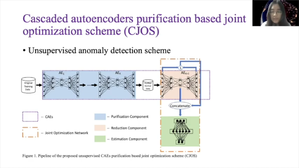
We cascade several autoencoders to act as the data purification component, which is capable of filtering out anomalies from unlabeled data, after case autoencoder filter. The data can be recognized as pure enough normal data with negligible anomalies. Then one more autoencoder is utilized to act as a dimension reduction component. And DNN is used to estimate some parameters of Gaussian mixture distribution. The last autoencoder and DNN is joined together to construct as a joint optimization network.
In detail, the cascaded autoencoders filters act as unsupervised data purification components. The training data is fed into the first autoencoder. After training we sort the data according to the reconstruction arrow between the input and the output. Here we use mean absolute arrow as the measurement metrics. Then we draw out a percentage of the data with another reconstruction arrow as potential anomalies.
The remaining data is fed into the second autoencoder and repeats the formal steps. After a few runs of autoencoder filtering we can gather the data set with only normal data. Actually, we have demonstrated this unsupervised data purification effectiveness, both theoretically and empirically in our previous paper. And as experiments we get our best performance in which case is that [inaudible] R is that 20 percentage.
Here we go to the joint optimization network, which consists of the last autoencoder and DNN. So DNN can be expressed as this function: where P is input samples, W is a weight matrix, B is BIOS vector, sigma is a soft max activation function. And P hat is output, which is a three-dimensional vector used for mixture membership estimation. We use output of DNN to estimate the parameters in the Gaussian mixture distribution, we see Gaussian components.
Then also may uncover [inaudible] matrix of the theory [inaudible] component as mu C, and sigma C, and as the probability that the sample belongs to the Gaussian component as alpha C. We estimate the parameters in Gaussian model as its formulas will, and prime is a number of input samples, Pic hats, as a probability that why it comes from the CAEs component. We connect to the last autoencoder and a DNN retrieves them jointly.
So input of the last autoencoder is original input features and input of the DNN consists of two elements. One is the middle coded the layer of the last autoencoder. Another one is the reconstruction arrow between the outputs and inputs of the last autoencoder. So objective function for joint optimization network contains the loss function of autoencoder and the sample energy of DNN. And EPI is a sample energy, which is negative log probability of observing the input sample PI.
This joint optimization is used to solve low [inaudible] problem. For testing sets we calculate their sample energies as anomaly scores. And record the probability of solving input samples as a PI with confidence, which we will use in the following steps. All the steps with anomaly scores, ladders and threshold will be treated here as suspicious anomalies. So threshold is that according to cross-validation step.
In the following I’ll introduce how we extend our, the proposed unsupervised anomaly detection scheme to the insider threat prediction problem. Before that I will introduce the dataset we used in our experiments to show how our work can be utilized in practice. It is a collection of synthetic insider threat test data sets published by CMU. It is only available data sets for public access. It is several versions. We use the latest version, r6.2, which contains the most complex situations.
There are a total of around 120 gigabytes system operational files recording for solving employees’ actions about device connection, email communication, web browsing, file printing and log on. The log of activities was within 516 days. Employees’ metadata information are also provided.
LDAP directory and psychometric file store the functional information of current employees in each month, as well as their big five personality traits measured by the corresponding psychometric scores.
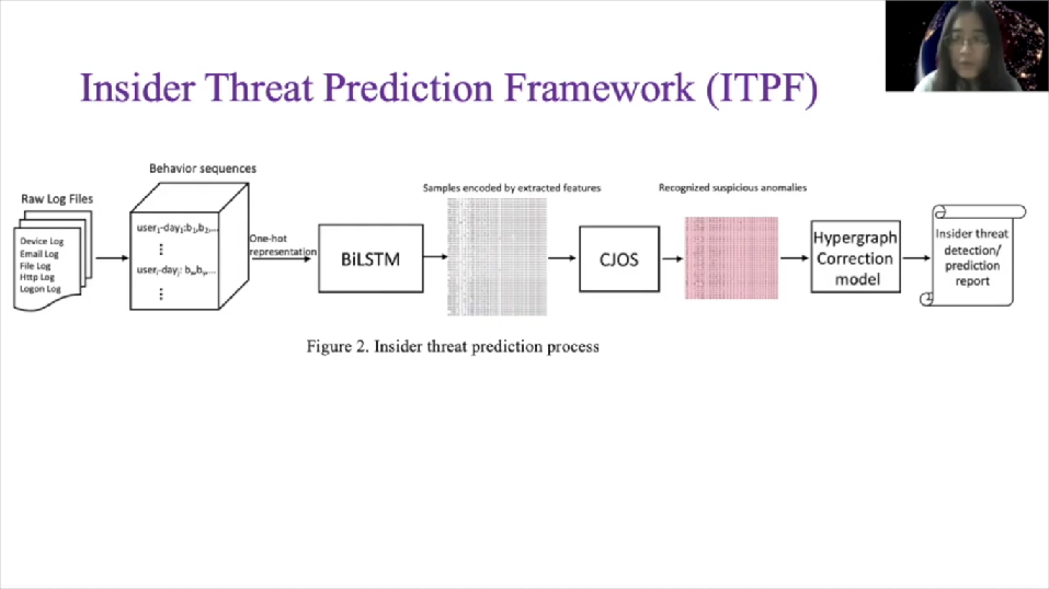
This is the workflow of our Insider Threat Prediction framework. What we have is a raw log files as I mentioned before. We pre-process that dataset. And for each user in each day, a behavior sequence is generated. Each behavior sequence is a sequence of numbers, which represents the employee’s actions chronologically. And after generating the behavior sequences, we feed it into BiLSTM model to learn the behavior language of employee’s actions as an LP task.
After training, we use the last hidden layer of the BiLSTM model as the extracted features, and the samples encoded by extracted features are then fed into CJOS. After the formal training steps, when your behaviour records come, then we’ll go through the formal steps and CJOS can recognize the suspicious anomalies and give out an anomaly score for each sequence, with the help of Hypergraph correction model. The behavior sequences, we use a correction confidence less than the threshold where it’ll be predicted as insider threat behavioral sequences. Therefore we can respond in real time and eliminate the insider influence as soon as possible.
Let’s go into the details. So the first step is about how we pre-process the raw log files, encode them into the input of the BiLSTM feature extractor. We combine the log entries from each log file on the per user per day basis and arrange them as behavior sequences according to the timeline. We investigate the user’s daily behaviors in the context of this dataset and extract a total of 164 behaviors numbered from one to 164, respectively, as listed in this table.
Select one value in each row to construct one user behavior encoded with a number, for example, connecting a device in the office hour at weekday is encoded with one. And the corresponding is connect operation is encoded with two, et cetera. For each user each day there is one behavior sequence after this pre-processing. A total of 1.3 million behavior sequences are generated.
BiLSTM is a variation of classical LSTM model in different ways of autoencoder. LSTM is not a feed for one network. It has loops. During training so input of the latter units as related to the alpha state as a former unit. BiLSTM still has the basic LSTM units. And it has two directions – forwards LSTM and backwards LSTM. Given an input sequence, we use one hard encoding to embed each factor BI, to a vector VI and then feed into the BiLSTM as one of the input samples. The BiLSTM model can predict the output of VI as YI.
And the last function is binary cross entropy between BI plus one and YI. After training, we use the hidden states of the last hidden layer as learning features. Users’ metadata features, for example, show supervisors’ psychometric test score, et cetera, are concatenated with [other] features to form the final extracted features. Then all the samples encoded with these extracted features are fed into our CJOS.
Then we apply our CJOS to do insider threat detection prediction. The outputs of CJOS contain all input behavior sequences, probability of them conforming to Gaussian Mixture distribution, and the stats of suspicious behavior sequences, if they’re corresponding and other scores are lighter than the threshold.
So output probability is considered as a [inaudible] probability of corresponding examples. Through experimental evaluation, we can catch almost all insider threat behavior sequences through our formal steps. However, because we would also drop some parts of normal data during the data purification process there may be not enough normal data to estimate the Gaussian Mixture distribution, which would lead to high false positive rating issues.
So we add a hypergraph correction module to improve the detection and prediction accuracy. Hypergraph is a special kind of graph compared to traditional graph, hypergraph also has a vertice and apse, which we call then hyperapse.
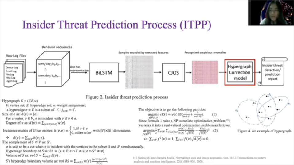
One of the differences between the hypergraph and the traditional graph is that one hypergraph can contain more than two vertices. Take figure four as the illustration, you want [E2 and E3] hyperapse which contain more than two vertices. As this is a pure mathematical problem, due to the time limitation [inaudible] the complex mathematical definition and the detection and introduce how we use spectral hypergraph partitioning to help us distinguish a true positive from false-positive insider threats.
After the spectral hypergraph partitioning, we can get two partitions and we call the partition with smaller size as hyper abnormal partition HA and the partition with larger size as hyper normal partition HN. So records in HN, adds the correction confidence with the value of phi multiplying, corresponding appearance confidence, and those ones in HN gets a correction confidence with the value of tau, multiplying, corresponding appearance confidence.
For better ease of corresponding appearance confidence we obtain our proposed CJOS scheme. Hence we can give out a brief confidence of each recognized suspicious anomalous sample, being the actual insider threats. For users without domain knowledge, we start a threshold eta for them to make a final decision, where eta is set according to cross-validation procedure, they can predict the behavior sequences as actual insider threats if they’re corresponding correction confidence are less than eta.
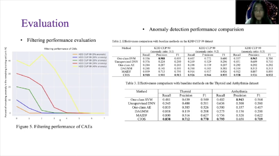
We evaluated the nominal detection performance of our CJOS on some public benchmark datasets. Figure five shows the filtering performance of our cascaded autoencoded filters. Lines with different colors, represent a model working on the data sets with different anomaly ratio. They are showing the decreasing tendency of remaining anomalous percentage in the remaining training sets, also encoder and autoencoder.
That also shows the value of K required to filter out all those anomalies in the training sets. One autoencoder is enough to purify the training sets when an anomaly ratio is less than five percentage. And even if the anomaly ratio is increased to 40% our scheme still has a capability to purify the data with unsupervised manner.
For the anomaly detection performance evaluation we use a standard evaluation matrix, recall precision and F1 score in the table one, two, and three. For each column the best result is highlighted in bold. CJOS almost achieved best performance, although one class of VM gets slightly higher precision, it suffers quite low recall and F1 as sacrifice, which are unacceptable in real cases.
About insider threat prediction, performance evaluation, we use three metrics: Recall, False Positive Rates, and AUC. Recall shows the ability of discovering the actual insiders threat behavior sequences. For insiders threat prediction it is critical to discover all those insider threats in the organization, things even one overlooked insider action will bring huge damage to the organization. Therefore recall also the same as a true positive rate is the most important matrix [metric] for insider threat prediction, performance evaluation.
Meanwhile, too much false alarms will cause much work load for digital investigators. So false positive rate is another digital metric to your various methods, as true positive rates and a false positive rates is a pair of trade-offs. We also look at AUC score, which indicates area under the ROC curve. Whereas the horizontal axis represents the false positive rate and the vertical axis denotes the true positive rates.
So best metric results have enabled in bold in table 4. Through experiments we demonstrate that our insiders for our prediction framework outperforms other state of the art baseline models. The false positive rates in the proposed framework is less than one quarter of the smallest of false positive rates achieved in other baseline models. Additionally, our insider threat prediction framework acquires higher recall and AUC score than the state of the art deep learning methods.
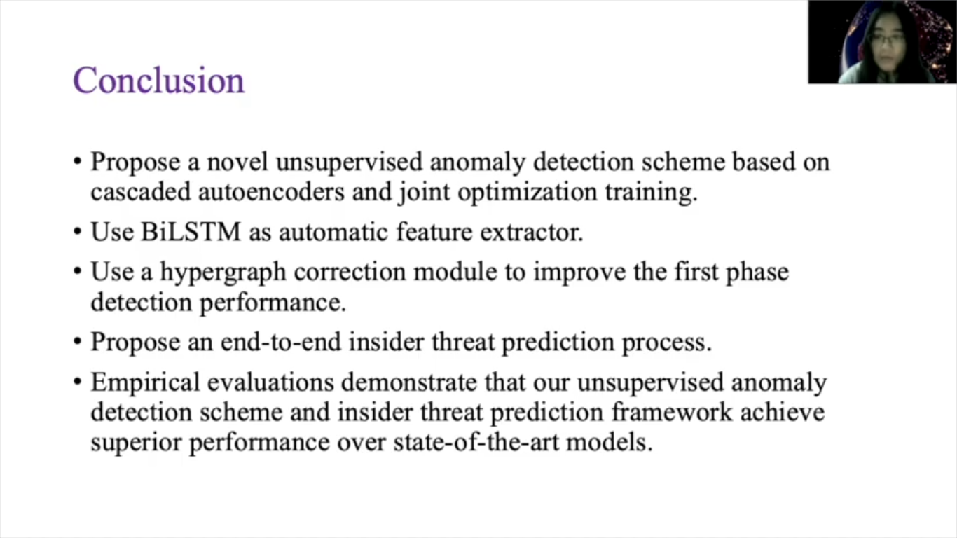
About the conclusion, in this paper, we propose a novel general unsupervised anomaly detection scheme based on cascaded auto encoders and joint optimization at [inaudible]. Our core idea is to utilize cascaded autoencoders to do data purification on all unlabelled data, then join to the optimizer dimension reduction and the density estimation network to avoid suboptimal problems.
On the basis of this scheme, we design an end to end insider threat prediction framework for proactive forensic investigation, through which we can make real time response to prevent the harmful influence of insider threats. We extracted those scalable feature representation automatically through the data-driven BiLSTM feature extractor, waving the time consuming feature engineering work. Additionally, a hypergraph correction model is applied to solve the common existing relative high false positive rate problem inside forensic detection. We evaluate our scheme and framework on public benchmark datasets.
The experiment demonstrates that our models outperform state of the arts unsupervised methods. About our feature work for automatic feature extraction we use BiLSTM as a feature learning model, which is capable of catching temporal relations between actions.
However, the context of the actions is also important for future extraction. So in the next step, we will try to use BERT learning model as the feature extractor to see whether the performance can be raised or not. Till now most existing, deep learning solutions for anomaly detection problem can only work for structured data and ignores the underlying relations among the data. Our next work will take use of Graph Neural Network to improve the performance.
Since autoencoder has shown its strong capability in unsupervised learning and the dimension reduction and there are already many variations for autoencoder we will try to utilize its advanced variations for automatic visual extraction, and as I mentioned reduction, for improving the performance and accelerating the training speed in our future work.
So that’s our presentation today. Thank you.


