Hi, my name is Anh Duc Le. This is my honor today that I’m going to do a presentation for our team, introducing a new algorithm named ChunkedHCs, used for the authorship verification task. The algorithm is tested on Reddit users as our case study.
So talking about team as well, why this paper exists at the first place. Half a year ago, I was a master’s student in Ireland. And I was doing my master thesis at the time, the topic is this very topic. This paper was submitted to the DFRWS conference. So my academic supervisor for my dissertation was Dr. Justin McGuinness. He is the lecturer at Minster Technological University in Cork, Ireland. And I really love his teaching. He supported me a lot while doing my master’s.
The second person behind this work is Mr. Edward Dixon who is now my boss, he’s the founder of the Rigr AI. He’s really fascinated about the forensic [indecipherable] sensitive data. You could contact him via his email for interest indications about forensic and sensitive data. Finally is me, Anh Duc Le I’m the machine learning engineer at Rigr AI, also the lead author of this paper.

So let’s talk about the next thing, what does it do? We started a very simple questions. There’s many so-so [indecipherable] platforms like Facebook, Twitter, Reddit, etc, and how to know which accounts are duplicated? And why does it matter?
Because finding true people behind fake accounts used for illegal activity is the objective of the academic researchers in district practice in the, in legal enforcement officers working in the digital forensic domain. So turning to the objective of the paper is to identify whether to a social media can belong to the same person by examining if their comments and posts are from two accounts is the authorship verification task.
So authorship verification could be classified into intrinsic or extrinsic. So in this way, we focus on the intrinsic method. So there’s going to be different paths, approaches, but there’s one problem. They all involve complex feature selection and sophisticated pre-processing steps.
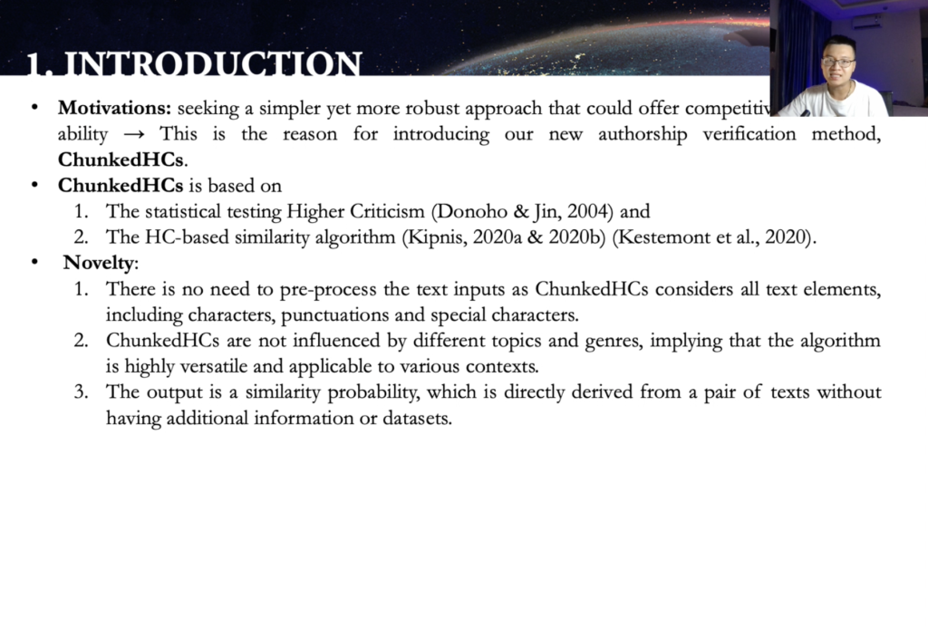
So this it the motivation for us to introduce our new algorithm, ChunkedHCs. And ChunkedHCs is based on the statical testing, higher criticism and SCBA similarity algorithm. So the novelty of this study is going to be, there’s no need to pre-process texting, but as ChunkedHCs considered all tech elements, including characters, punctuation, and special characters. And ChunkedHCs are not influenced by different topics and genres, and the algorithm is highly versatile and applicable to various contexts. The output is a similarity probabilities, which is directly derived from a pair of texts without having additional information or data sets. So the computation is quite light as well.
So here, our research questions. Now we are going to talk about, first thing first, the theoretical foundation of the paper, and the [indecipherable] first. So it’s a statistical test to test a very subtle problem from a large number of independent statistical test, all of the null hypothesis are true, or some of them are not.
Suppose we have the set of N P values from P1 to Pn. P1 is the smallest and Pn is the largest. And the [inaudible] are device follow. When HC are launched, the setup heavily inconsistent of the global known hypothesis, which means there’s enough evidence to support the global alternative hypothesis. From the HC objective function and the HC statistics, the index i* star. So when the HC is maximum and corresponding with the THC, which means the HC threshold, are defined as followed.
So phase four is going to be very useful for feature selection in the classification settings. So we’re going to know settings. So, okay.
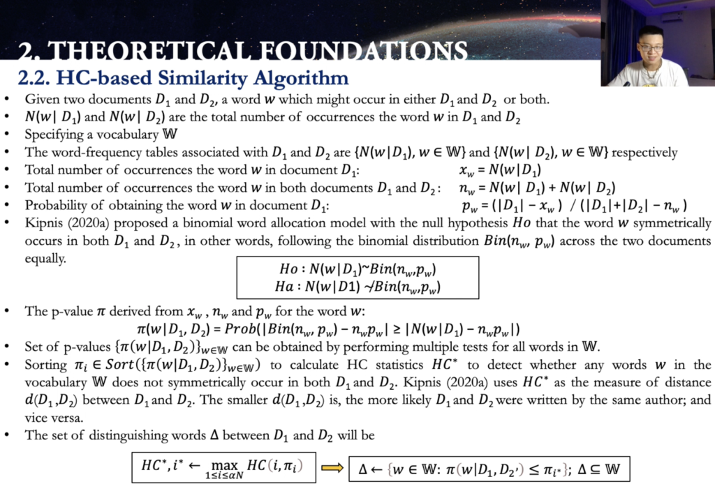
And about the next step the next theoretical base for the ChunkedHCs, which is the excavator similarity algorithm. So there’s going to be a lot of notation and equation for this algorithm, but in short, [indecipherable] 2020 proposed a binomial altercation model, and to use that model to measure the distance between two documents by using the EXIF statistic if the distance between two document or the EXIF statistic is large. So two documents are different. And if two, the distance is more, so two documents is going to be the same.
Also here from the [indecipherable] by calculating the statistics, he also derived the Delta term, which is the set of the the author characteristic [indecipherable]. It’s a very important property of the HC based similarity algorithm. So it’s automatically focused on the author [indecipherable] recent word, rather than the topic word, the algorithm is that robust and suitable to deal with the authorship task in different topics.
Now. So it’s the HC based similarity algorithm summarized in the algorithm format. Right. So we’re now going to talk about the ChunkedHCs, the next slide. So now I’m going to talk about the ChunkedHCs algorithm, which is the meat of this presentation, the research.
There’s going to be three steps: step one, chunking the texts; step two, measuring HC distance between chunks and corpora. Step three, estimating similarity probability.
Now talking about step one, given paths like T1, text one and text two, each of them split into chunks of identical lines of the characters. That line is going to be C.
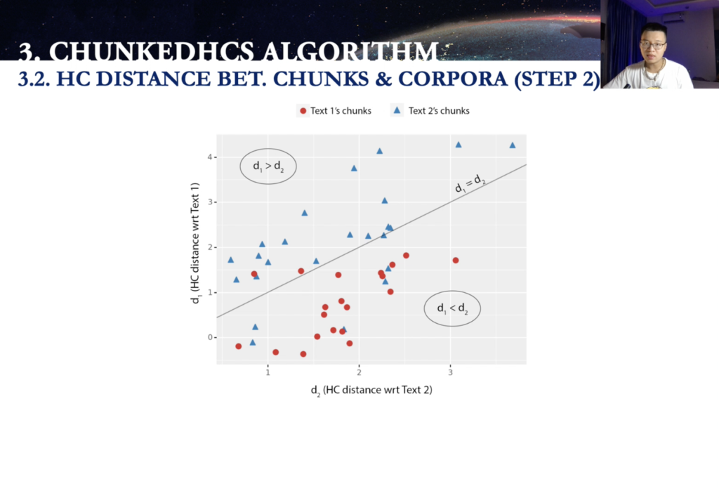
So, yes. Now talking about step two, we’re going to measure the HC distance in different chunks. Now we have divergence of each of the text one and text two, let’s say in this case, text one is red, text two in blue, all together in this 2D coordinate, but I’m going to explain to you why those [indecipherable] chunks are placed in those positions right now.
So we have like a TK is individual chunk in this case. So you can see the yellow one here. So cool. The chunk [indecipherable] is the text teaching. So dK, we measuring the distance between this chunk with the off the cut of the [indecipherable] versions from text one. So d1k and also the d2ks, these chunks with the rest against, with same kinds. I mean the blue one. Yeah. So d2k and d1k. We have those.
And then now we compare the distance. If, in this case, d1k is larger than d2k. So it’s going to be classified that dk is categorized as the [indecipherable]. And we’re going to do for all the rest of the individual chunks here. And we got the, so the number of C1 press, plus the number of C2 press, equals the number of C1, plus number of C2.
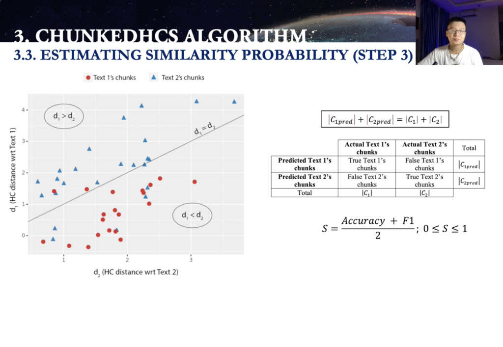
Now, what are you going to do next? Estimating similarity probability? No. So after doing the classification, so separating, you can see here, the [indecipherable] is where do you want [inaudible]? So for the rest, so above this [indecipherable] is D1 larger than D1. Those are gonna grow up into the, the C2pred and those below C1pred. And we can have the confusion matrix between among the actual classes and predicted classes, and we can derive from here, the accuracy and F1 to calculate a score here. In this case, score is ranging from zero to one. Now there are two possible extreme scenario in this score.
Let’s say the text one, text two, two different authors. The, the first extreme scenario here is the, all of the chunks are separated clearly. And then the accuracy and F1 in this case are both 1N leading to the [indecipherable]. Difference going to be one. So they’re not extreme scenario is technology that takes to assume they are from the same author, and then all of the [inaudible] are going to be missing them altogether.
And then in this case, accuracies and F1 both [inaudible]. So in this way, we have [indecipherable] similarities also is the [indecipherable]. And now we have the S score here. So it’s the average written accuracy and F1, and we can plot it into the graph like this, and the two extreme scenario, one a design difference, and one a design similarity. And then we turn it into probability like this. So, and then we, we just little bit kind of the transmission and the conversion here.
And we do have the… we can calculate the probability similarity in this case, derived from the S score. In this case when [indecipherable], which means the popup similarity probability, when it to one indicate a [indecipherable]. So the text one and text two [indecipherable] from the same author when the similarity probability is approaching zero. So it’s indicated those [indecipherable] from two different order.
So the [inaudible] can summarizing like this. They might be three steps: step one, step two and step three. So the input is the step one, the text one and text two, and the output is going to be the similarity probability. If that’s going to be one, so texts one and texts two are from the same author. If the similarity probabilities is approaching zero, so text one and text two are from different authors.
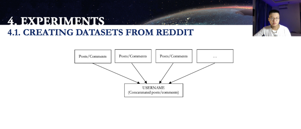
Now talking about the experiments and firstly let’s create some datasets from Reddit. We’re going to concatenate the kind of aggregate posting common for that one user name. So for his or her, so create a power of two different nodes by using two different usernames. So that just the assumption, they actually from two different people, because we cannot validate and verify whether or not they are actually from the same or different people.
So create a pair, the same author. So we just only use one username and split it into two halves. So now we’re going to create some dataset for surveying and testing, and surveying is going to have the the short texts and long texts. [Indecipherable] in our studies should consider having less than 10,000 characters. And [indecipherable] are more than 10,000 characters. For each of the interval, the number of pairs of similar and different authors are equal.
And then, so for serving ChunkedHCs, to find the perfect combinations of the vocabularies and the chunk size. So to have the best performance that we could have for the testing now for surveying ChunkedHCs. And this is for the [indecipherable] for texts between 1000 and 10,000 characters. This is the heat map for the [indecipherable] score for different trends in vocabulary size. First thing first, ChunkedHCs, they have poor performance for chunk sizes of 100 or 200 characters when it’s only slightly better than random guessing. The AUC score is just above the [indecipherable], meanwhile, the largest transfer of 3000 characters [indecipherable] all the smaller chunk size.
Interestingly, the combined intelligence of five characters with the vocabulary side of 20 most frequently used will provide the best result for [indecipherable]. So here is the 10th combination of the ChunkedHCs and vocabularies size, which in which an essay has the highest score for the entire [indecipherable] success. So we can see that there are short chunk size, and 500 and 800 characters could be the suitable charge for tests between 1000 and 4,000 characters. For testing between 4,000 and 6,000 character that’s missing, or [inaudible] for texts between 6,000 and 10,000 characters. The chunks at 2,000 characters offer good resolve for all cases.
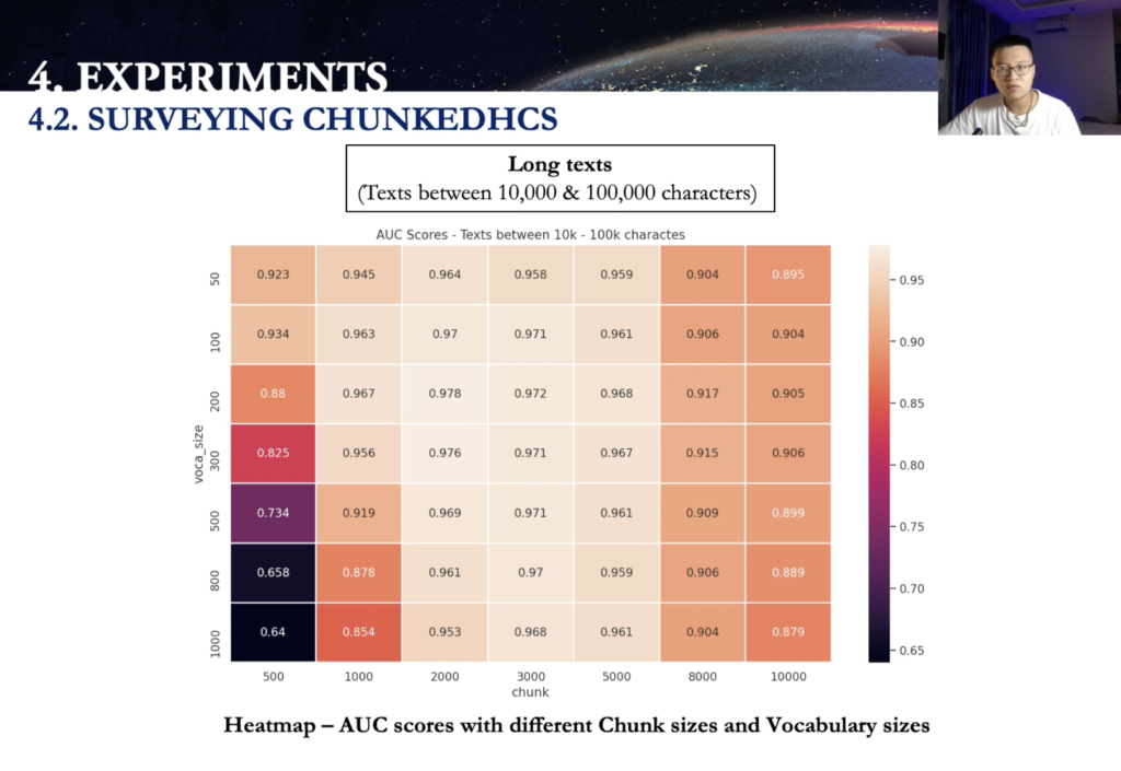
Now talking about the long texts between 10,000 and up to 100,000 characters. So this is also the heat map for the AUC score for different genes and vocabularies size. The chunk size show poor performance for the shortest [indecipherable] size of 500 characters with the vocabulary of 200 to 1000 more for any frequently used words. Performance decreases when chunk size is greater than 8,000 characters, the algorithm had the desirable performance with the chunk size around two, three and 5,000 characters.
Now talking about the AUC score for individual intervals. So this really illustrate the AUCs for the all interval from 10 combination of the chunk size and vocabularies size, where the algorithm has the highest AUC score for the entire long text assess. So there’s some fields of vision here. First, a lot of that text corresponds to a higher AUC score generally. Second, the only sub two difference for the AUC score among the combination of the chain side and the vocabulary size for all the intervals, in particular [indecipherable] difference becomes smaller and smaller with the texts.
Now, we talk about testing. So from the surveying the ChunkedHCs, we just know the combination of the chunk size and the vocabulary size. Yes. [indecipherable] Now this session is testing the algorithm by using those is that choice from [inaudible] from the previous session for the text from reaching the ranging from between one to 2000 characters to between 29 to 30,000 characters. For at least the selected values of chunk size and vocabulary size, the similarity probability is calculated for all the stuff is step one. And next, the data set is written to two [indecipherable], which are the validation set, and the test set for each interval, the valid insight, a useful facility, optimal threshold, where accuracy is maximum and the final step here.
So we on the test [indecipherable] we use [indecipherable] to predict the positive and negative class, and then classification metrics, including accuracy [indecipherable]. And I used [indecipherable] for individual intervals. So over this session I provide a detailed picture of the algorithm ability and its limit.
Now, talking about the chosen… so this is the density plot, or similarity property distribution for all of the intervals. So with the chosen chunk size and vocabulary size, the similarity probability is calculated all of the [indecipherable]. This will demonstrate the similarity [indecipherable] for the pairs of both similar and different authors.
So there’s three observations here. The [indecipherable] below 10,000 character tend to have multimodal distribution for texts about 10,000, for texts above 10,000 characters. So the similarity [indecipherable], it had the uni model distribution. As the texts get longer, the distribution of the two classes become more and more distinct. Within the scope of this, the accuracy at the [indecipherable] classification metrics quantifying how well ChunkedHCs identify pairs of similar authors. This is the basis for choosing the decision [indecipherable], but accuracy has got a maximum on the validation set. This [indecipherable] how the threshold value chains across the text lane for interval between the one and 6,000 character, the decision thresholds are larger than the author threshold value. For longer text threshold value of [indecipherable] threshold value [indecipherable] five.
So talking about the testing, the ChunkedHCs and the test set. So with the optimal threshold derived from the validation set, [inaudible] predicted on the on the test as the table and the light light graph show the AUC accuracy and F1 score for all of the intervals. Firstly, for all, for the shortest interval between one and 2000 characters, the accuracy F1 are around 0.645 and 0.7 respectively. For texts between 5,000 and 10,000 characters, the accuracy is above 0.7. For longer texts, the [indecipherable] metrics increase. In particular, the accuracy [inaudible] three respectively for the log is that between 29 and 30,000 characters.
Now we talk about discussion, the input, the algorithm does not need to require sophisticated pre-processing steps. The ChunkedHCs could be a [indecipherable] case suitable for authentic, which lie of author and English, and also being suitable for authors’ social media platforms such as Facebook, Twitter, etc. ChunkedHCs might not adequately capture authors’ writing styles due to the distribution of the [indecipherable] that in under represented features would potentially cost the algorithm verification ability. So it’s advisable to consider the imbalance class when applied in the ChunkedHCs.
So recommended: there should not [indecipherable] this one, between the texts level for the two texts in [indecipherable], avoid the bias in the internal binary classification for the outputs. So ChunkedHCs directly derives, similarity or abilities, zero indicates power of different author. One indicated power of the same author, but in most cases, might be more challenged to conclude with less definite probability values. So the [indecipherable] for the authorship or against verification task in choosing a universal threshold, these things wishing the positive and negative [indecipherable]. So threshold might need to be attributed for different data sett also depend on other factors.
Now talking about the performance. So ChunkedHCs provide good results when texting, but as a sufficiently long, it crucial to carefully select the chunk size vocabularies are in this decision pressure for different unique lens. So from the empirical results, shortage [inaudible] should be small and decision threshold needs to be more conservative value, closer to upper limit of one for longer texts. The chunk size should be approximately 2000 to 3000 characters, with common threshold at zero five.
So for the runtime, the ChunkedHCs is fast and straightforward without having training that or measuring the AC statistic has a moderate computational cost. And ChunkedHCs will be slower with the longer texts or having shorter chunk size with the larger vocabularies size.
Now comparison with other approaches. ChunkedHCs offers much similar [indecipherable] than machine learning or deep learning approaches. Nevertheless, it might come because at the verification ability, suggestion say performance might not be as good as this. This is only the brief preliminary papers as the introduction to this topic. And there are a [indecipherable] them was not [indecipherable] compared with all the other shift verification approaches.
So talking about the conclusion and future. So ChunkedHCs is the algorithm specifically designed for the authorship verification tasks. So ChunkedHCs is going to give a similarity probability from 0 6 1 0 and decay a different the power of different author and indicate a pair of the same author. And then applying ChunkedHCs on 30 users that task going to be… so the problem is going to be much be improved for the texts that are longer. So especially, [indecipherable] 0 9 4 4, the text between 29 to 30,000 characters.
And for the future works. So we’re going to [indecipherable], sharing some similarity. So mapping all work to the corresponding part of [indecipherable] speed task. There’s some modification for the tech input with this, the things that our team now currently do in this show, promising results and optimizing the key parameters, and also expand this study to to other data sets and comparing ChunkedHCs to other approaches.
Thank you for listening.