Hi all, thank you for your interest in this presentation that will cover the research work conducted by myself, Cezar Serhal, and Dr An Le-Khac from UCD. Our paper presents a machine learning based approach to triage smartphone content using file metadata. In this presentation today, we will cover our problem statement, the research objectives, some of the related work, the adopted approach, the obtained results, and finally we will wrap up with a conclusion and possible future work.
So we start with the incentive for this work, which can be split into four key factors. First, the high mobile phone penetration, which exceeds 90%. This results in law enforcement agencies facing an increasing number of cases linked to mobile phones. In addition, the increasing storage capacities of mobile phones, which should reach around 83 gigabytes on average in 2019, and the focus of existing extraction and examination tools for finding all the evidence.
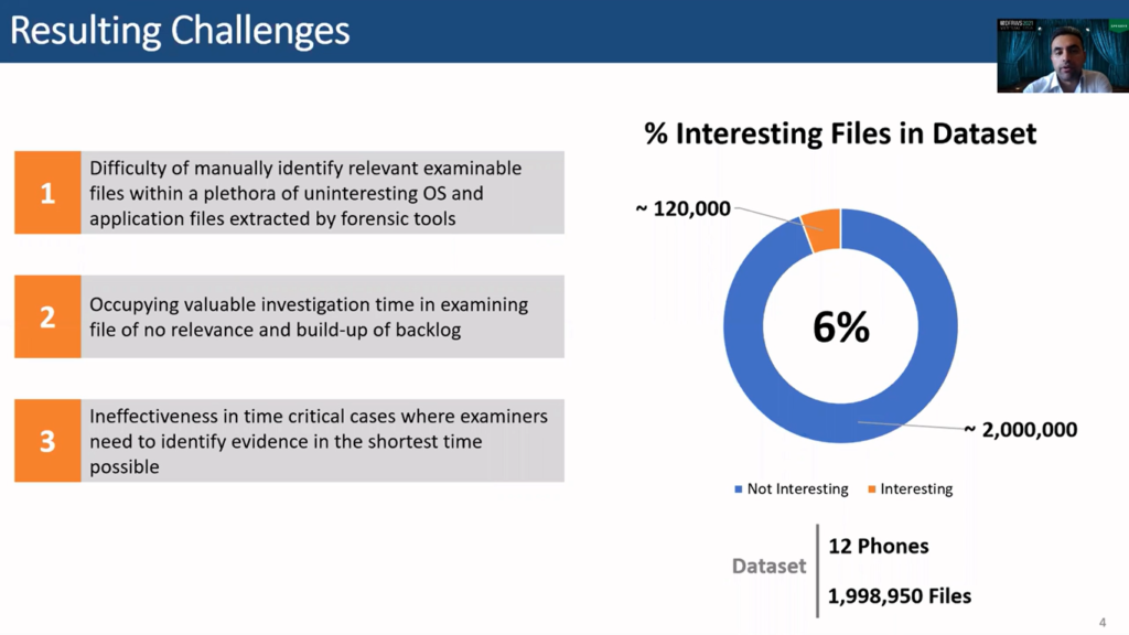
All of this results in presenting examiners with a large number of files, most of which have no added value for the investigation. This can be seen, for example, when consulting the dataset used for this research, which consists of around 2 million files accepted from 12 devices, where only 6% of the files were of interest for the examiners.
Thus, manually examining all extracted files takes up valuable investigation time and occupies skilled resources in examining files of no relevance. In addition, this approach is ineffective and time consuming, in particular for cases where examiners need to identify evidence in the shortest time possible.
To tackle this issue triage techniques can be used to classify files based on their possible interest. More specifically, automated tools that embed the examiners knowledge and skills can be useful to perform this task. Several digital forensic triage methodologies based on classical automation techniques, such as block hash and regular expressions profession matching have been proposed.
However, such techniques suffers from the significant limitation of requiring law enforcement users to know and hardcode data templates and relations of interest beforehand.
More flexible machine learning based approaches have been proposed. Some researchers specified whether a device is of interest based on its usage metrics and file metadata (mind you, this is about classifying devices, and not files).
Other researchers applied machine learning on files and system metadata to identify the owner or carved data, or to identify malware. Only one recent research proposed a machine learning approach to classify files based on their metadata.
Moving on to the research objectives. So, we aim at answering the question of whether a file metadata and machine learning can be used to decide if a file extracted from a smartphone should be examined or not.
The research question is built upon the hypothesis that file metadata can indicate the relevance of a file for an investigation, and that machine learning classification algorithms can actually model the decision-making process required to identify files of interest. And finally that different classification models will perform differently.
So, moving on to listing some of the relevant work in the literature, we can see that several approaches were proposed to identify if an examined device is relevant to a specific crime using machine learning classification algorithms. Applied on device usage information, such as the number of holes and a number of videos, numbers of photos and other metrics. Among those are, for instance, Martuana et al. and Gómez.
Dalins attempted to automatically label child exploitation material based on the content and not metadata focus using deep learning. In 2019 Du and Scanlon presented a machine learning based approach for automated identification of incriminating digital forensic artifacts based on file metadata, which is very similar to what we’re doing.
However, the experimentation results are based on files generated and extracted from computers and not from smartphones. The adopted approach leaves also room for enhancement in some areas, such as feature engineering, feature selection, and hyper-parameter tuning.
The important thing is that the results show that performance is affected by the prevalence of the class of interest. This highlights the importance of using data similar to real world cases in order to generate classifiers that are effective in practice and not just in theory.
The use of machine learning on file metadata in digital forensics is not just restricted to the triage field. It is also used to answer other similar questions, including ones that, in essence, are classification problems.
For instance, Garfunkel et al. in 2011 presented a solution to identify the owner of data carved from storage devices used by multiple users. Muhammad in 2019 used classification algorithms to reconstruct cybercrime events based on file system metadata. Milosevic et al. in 2017 implemented two approaches based on machine learning algorithms to detect malware.

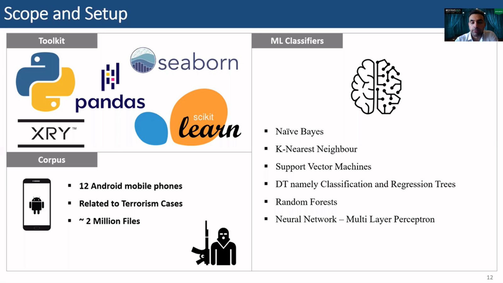
To implement and test the proposed methodology, we used the following software: Python, Pandas, scikit-learn, seaborn and XRY mainly. To narrow the experimentation scope, we only considered Android devices, which currently consists around 70% of the market share. Yet this approach should be applicable on other types of mobile operating devices.
And in terms of purpose, the metadata that was used is based on terrorism cases. These were specifically 12 Android devices that resulted in around 2 million files from these cases. Several machine learning classifiers were tested, including naïve Bayes, K-nearest neighbors, support vector machines, classification and regression trees, random forest and neural networks.
To do that, a forensically sound approach that does not affect the evidence was used. This approach consists of six main steps. The first is forensically extracting the data or metadata from the files then conducting pre-processing, assessing feature selection, hyper-parameter tuning, training and testing, and finally doing evaluation of the performance.
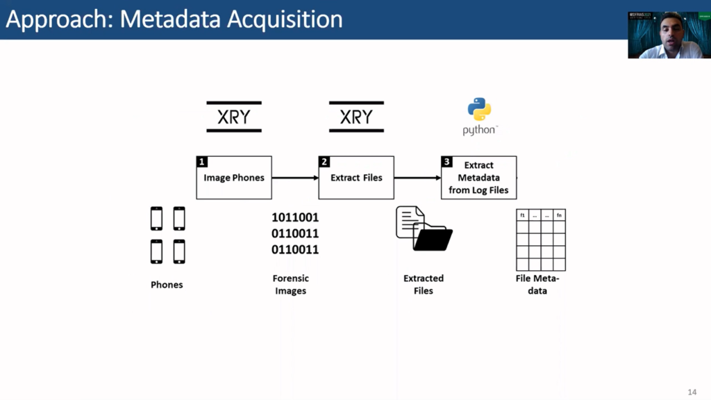
Starting with the first step, we start by imaging the phones, then extracting the files from the images, and finally using Python to extract the metadata that is locked in the extraction logs of these files. At this stage we are ready for pre-processing, which includes also exploring the data and labelling it.
To label the data, extracted files are manually examined by forensic experts, and then assigned to one of the following two categories: either a file it’s interesting or not is interesting. We consider a file as interesting if its content should be examined, and if it has comprehensible data.
Also a data cleansing strategy is adopted where records are checked for missing data and data variations. Variations are normalized, for example, file size units, and missing data is imputed if possible or dropped. Actual data records such as pipeline path and extensions are tokenized and encoded using CountVectorizer, which applies a bag-of-words approach.
Then the data is normalized by using a MinMaxScaler. This step results in a corpus size of 1,998,950 files. So around 2 million files.
Many features can be proposed for the machine learning models. In addition, the feature space can significantly grow after including adding code and category features such as path and extension. Training and testing a large number of irrelevant features on a large dataset could significantly affect the execution time and predictive performance of the models, hence one of the most challenging task is to identify the optimum set of metadata features. This is basically all feature selection.
To do that, we first consider our all available metadata to create a range of features, then feature selection is used to select the best feature set. Feature creation is influenced by domain knowledge, which helps reduce possibly irrelevant features for the problem at hand.
Accordingly, the following 12 base features are created: file type, file size, delta apprehended (which is basically the number of days between the the date of apprehension of a suspect and the file modified date for a certain file), an EXIF flag (basically to indicate if a file has EXIF data or not), the Xresolution, Yresolution (for photos), number of characters in a name, percentage of numbers in a name, percentage of underscores in a name also.
In terms of path, we consider the file path as text stream as a feature, the depth of the path (basically counting the number of slashes), and finally the number of dots in a path (which in Android devices usually refer to hidden files or folders).
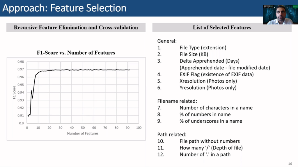
To select the best set of features, recursive feature elimination and cross-validation from scikit-learn library is used on the validation dataset. RFECV essentially automates the task of manually testing different sets of features to select the set that produces the best performance. RFECV starts with the complete set of features then eliminates the weakest features, then repeats until the minimum number of required features is reached.
As a result, all created features were selected while only dropping 12 out of the 75 vocabularies without a path. The dropped vocabularies are not base feature, and the figure shows that including them has minor impact on performance, as the graph slightly fluctuates around an F1 score of 0.969 after 23 features are selected, and then reaches a maximum of 0.9698 at 80 features.
To perform hyper-parameter tuning GridSearchCV from scikit-learn library is used to automate this process. GridSearchCV tries all possible combinations of the provided range of parameters with cross-validation and then selects the best. For our classifiers, this is the table of selected best hyper-parameters for our experiment.
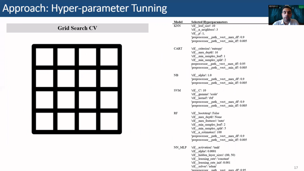
Looking at the selected hyper-parameters in our experiment starting with KNN, we see that a leaf size of 10 was selected, number of neighbors 3, and our parameter of 1 was used, also a maximum document frequency was of 0.9 and a minimum document frequency of 0.05. This is actually not related to KNN, this is related to the CountVectorizer, but this well within the pipeline, so we’re also setting its hyper-parameters within grid search.
For decision trees, we see that the criterion selected was entropy, maximum depth 16, minimum samples leaf is 1, then the minimum samples split is 2.
For naïve Bayes, alpha is 1, for SVM, the C is 10, the gamma is scale, kernel uses rbf.
For random forest, bootstrapping is not used, the maximum depth is not set, so they can grow. Maximum features are set to be auto. Minimum samples leaf is 2, but minimum samples split is 5, the number of estimators are 100.
For neural networks MLP the activation is tanh, alpha is 0.001, the hidden layer sizes used is 80 by 50, and learning rate is constant, learning rate initialization is 0.01, the solver is adam and that’s it basically…these are the selected hyper-parameters in our experiments.
The performance of the tested classification algorithms are compared, according to the following metrics: precision, recall, F1 score, and accuracy. As you all may know, precision is a ratio of true positive predictions out of all positive predictions.
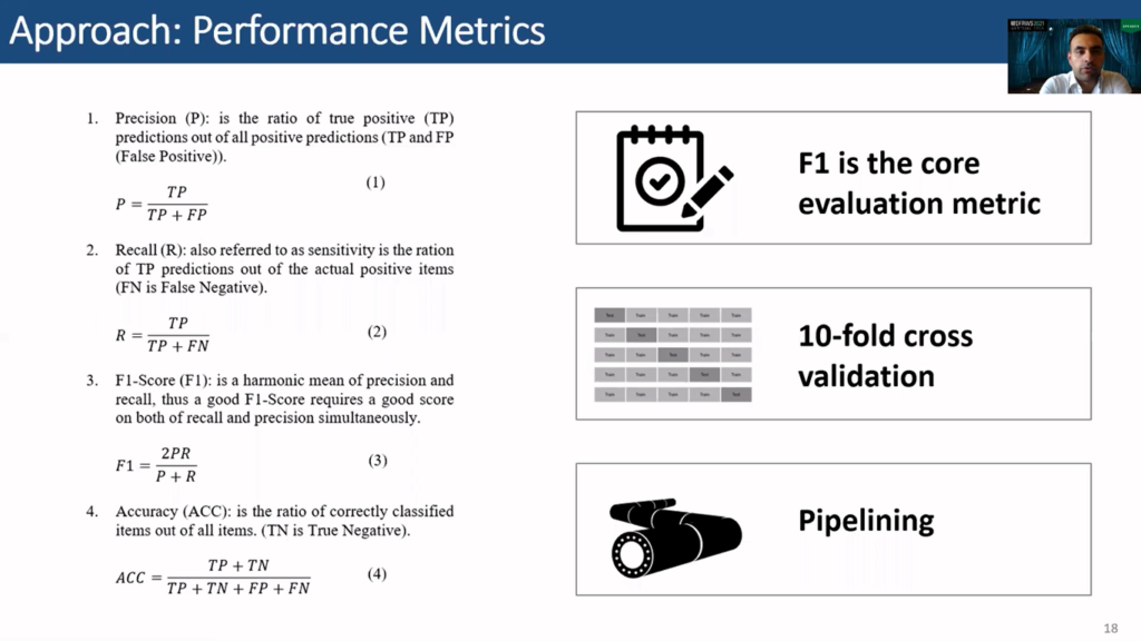
So in our case, how many of the files that are marked as interesting are actually interesting? This is a very important metric for us, as it indicates the precision of the classifier. A low precision means basically that we are bombarding the examiner with useless files for him to examine, and this defeats the purpose of triage.
Recall is also referred to as sensitivity, which is a ratio of two positive predictions out of the actual positive items. This basically means, or indicates, the performance metric for how strong the classifier is in actually recalling the important files, or the interesting files. A low recall basically means that we are leaving a lot of important files unmarked, and this will also create an issue for examiners.
F1 score is the harmonic mean of precision and recall, thus a good F1 score requires a good score on both recall and precision simultaneously.
Accuracy is the ratio of correctly classified items out of all items, and in cases where there is a class imbalance, like in our case, as we’ve seen, like 6% usually, (at least in our dataset, our files of interest) then this metric becomes less important. For instance, you can consider a very stupid…or a very basic classifier that always classifies files as not interesting, and in our case, this algorithm will result in around 94% accuracy.
The scoring measurement used in the cross-validation is F1 score, as it combines two important metrics for our case, namely recall and precision. A good classifier should be able to recall as much as possible of the files of interest, yet it should still preserve the precision to minimize the number of uninteresting files it falsely marks as interesting.
Also cross-validation is commonly used resampling method to characterize uncertainty in a sample, and to help assess the generalization ability of a predictive model while preventing overfitting. Thus in our experiments, we use tenfold cross-validation with stratified sampling to preserve class distribution in each sample.
Pipelines are also used with cross-validation to avoid data leakage by defining and applying a set of sample dependent pre-processing steps at each fold before applying the classifier. So for instance, normalization and feature encoding, which could be sample dependent, but these are bundled together and applied and reapplied at every fold of the cross-validation cycle.
So what are the results obtained from this methodology? The figures show the box plots of all the metrics obtained through cross-validation.
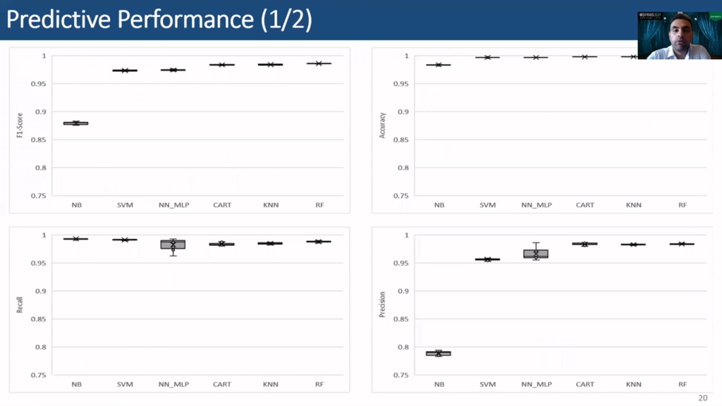
Classifiers show a consistent performance across metrics, achieving low standard deviation. We can see that a random forest achieved the highest F1 score at 0.9861, while naïve Bayes achieves the highest recall score at 0.9932, although it has achieved the lowest F1 score. This indicates that it did not perform well in precision, as can also be seen from the precision graph.
Random forest scores the highest precision at 0.9841, while naïve Bayes scores, as we said, the worst, scoring 0.7891. Random forest also achieved the highest accuracy at 0.9983.
Here are the results in a tabular format, since the objective of this experiment is to maximize both recall and precision so that the examiner is presented with maximum files of interest, while minimizing the files that are not interesting. The F1 score is used to rank the predictive performance of the algorithms for this research question.
Accordingly RF, or random forest, ranks first with an F1 score at 0.9861, precision at 0.9841, recall at 0.9881, and accuracy at 0.9983. KNN ranks second, CART comes in third, neural networks fourth, SVM fifth, and finally the naïve Bayes. All the classifiers except the naïve Bayes exhibit a very good classification and consistent performance, with an F1 score larger than 0.927.
Aside from predictive performance, execution time is worth considering, as large execution times can hinder model development efforts, or cause delays in deployment system. This slide shows the mean total execution time per cross-validation split.
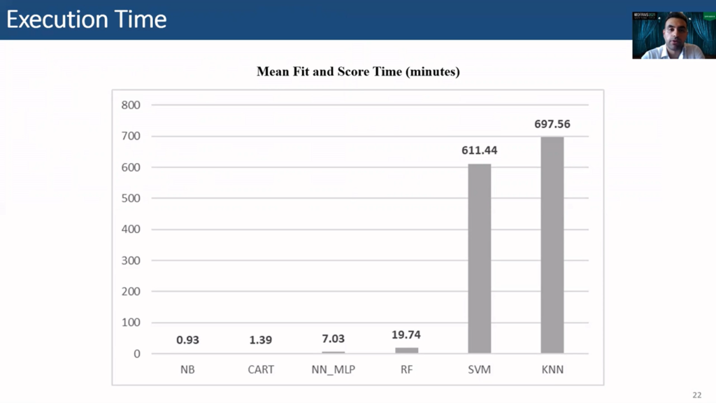
Mind you, this is dependent on the machine that the algorithms are run on, so these numbers might not be very useful on their own, but still they are relevant when we are comparing them to each other as all the algorithms are run on the same system. So we see that KNN is the slowest with a total execution time of 697 minutes, or around 11.5 hours. NB is the fastest with 0.9 minutes. Random forest requires 19.7 minutes on average at each cross-validation cycle.
So in conclusion, this effort validates the hypothesis that file metadata can indicate the relevance of a file for an investigation, machine learning classification algorithms can model the decision-making processes required to identify files of interest, and different classification models will perform differently with RF exhibiting the best performance in our case.
In terms of possible future work, this approach can be tested on other mobile phone operating systems, such as iOS, as it was restricted to Android devices only. Deep learning classifiers can also be tested and explored, and their performance compared to classical ML algorithms.
Finally, the effect of augmenting metadata features with features extracted from file content can also be explored. So not just relying on metadata, but also…well, creating features from the content of files, and seeing the effect that that would bring to the triaging files.
So this brings us to the end of this presentation. I would like to thank you all for your attention. And we are open to any questions. Thank you.