Bruce Nikkel: …paper of the session is from Jens-Petter Sandvik and his colleagues at NTNU, and it’s on “Quantifying Data Volatility for IoT Forensics With Examples From Contiki OS.”
Jens-Petter: Yeah. Thank you. So, I’m Jens-Petter Sandvik and my co-authors is Katrin Franke, Habtamu Abie and André Årnes. Yeah. I’m a PhD student at NTNU and in my spare time, I work with the Norwegian police in the Norwegian cyber crime center.
So, today I’m going to present a paper on measuring volatility by using Contiki operating system as an example. Here’s the outline of the talk where I start to describe Contiki and the file system, present a model for the volatility in the file system and show some experiments using the Cooja simulator. And wrap up in the end there.
So IoT systems are found everywhere today and everything, including smartphones and personal devices, industrial internet of things, and smart manufacturing and environmental monitoring, smart agriculture, smart infrastructure, power grids, and so on.
As the name suggests, the devices are internet connected either directly or going through a gateway. An IoT system spans quite a huge variety of devices from big clusters of servers running cloud subsystems to the tiniest devices with huge restrictions, both power consumption and on size.
Since there are many types of devices with a variety of constraints, there is also a huge variance in amount of memory and storage the device contain. The interface to these devices varies considerably: some have ordinary storage devices, such as SD cards attached; some can be read with ordinary protocols; while others have more obscure interfaces that requires specialized tools or knowledge for acquiring the contents of the memory.
The increased number of devices leads to an increased number of evidence locations, and together with a nonstandard interfaces, it leads to an increased resource demand if the data from all devices are to be collected in an investigation. If we can predict which devices that are more likely to contain data, the investigation resources can be better utilized.

So, from the background on the last slide, we see that one of the challenges is to do a proper triage, that is deciding from which device to collect evidence. And one of our challenges to that is to predict which devices still have data in memory. The probability for evidence in the devices depend on both the probability that particular device has contained evidence and volatility load: the data…how fast the data disappears.
In this talk, I will use “evidence” and “data” interchangeably, but with evidence, I mean, data that can be used as evidence for strengthening or weakening an investigation hypothesis.
The three research questions for this study was “how can data volatility in IoT devices be analytically calculated?” And “how can the data volatility in IoT devices be measured?” And “what are the differences between these two: the analytical method and the measurements?” How well does they correspond?
So, Contiki is an operating system for IoT devices and other resource constrained devices that needs very little hardware to run. The operating system was first released in 2003 and has been under active development since then.
To support low end hardware, the OS footprint is approximately 100 kilobyte and can run on as little as 10 kilobyte of RAM. It also comes with an emulator and simulator called Cooja (so that this shown here on the screen, the interface to that one), the emulator can emulate the hardware on which the OS image is running and the simulator can simulate huge networks of nodes and can connect to the internet through a gateway.
In this work, we mainly used the emulator to emulate the hardware and storage and single devices, so we didn’t focus on a network part of it. These protocols use IPv6. In addition, the OS Contiki contains IoT protocols, especially those defined by the internet engineering task force through various request for comments.
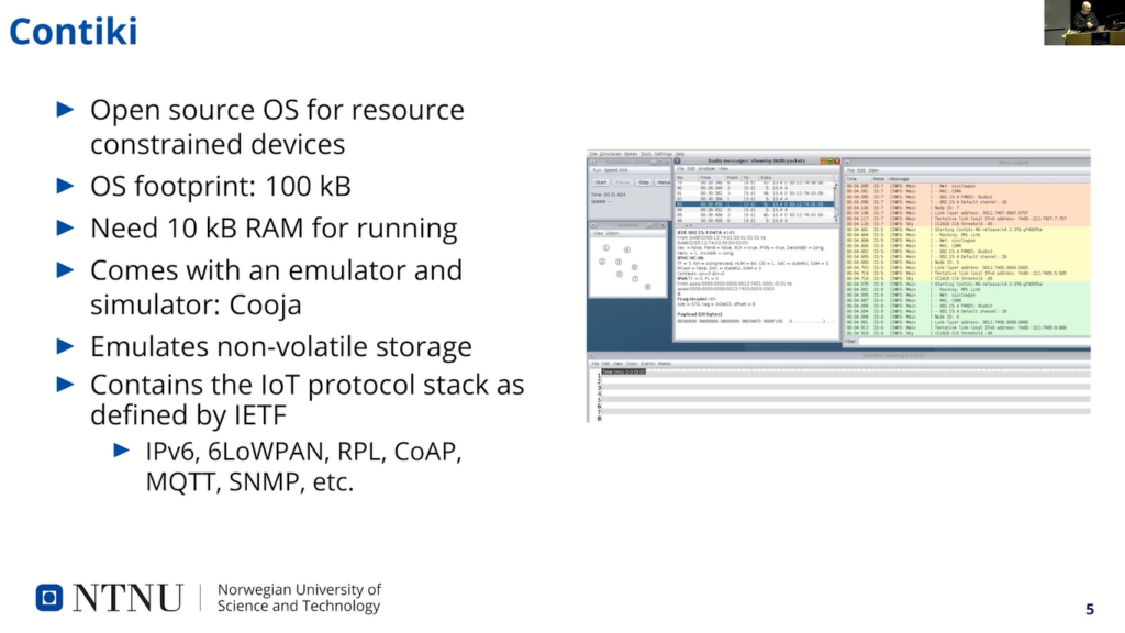
These protocols use IPv6 as a single network protocol and uses IPv6 over low power wireless personnel area networks (or 6LoWPAN) to send IPv6 packets over physical networks that don’t support a huge frame size. 6LoWPAN is also used in thread and matter protocols that has become more popular these days.
On top of 6LoWPAN, Contiki supports also routing mechanism called Routing for Low-Power and Lossy Networks, or RPL, and it have built in application protocols such as the constrained application protocol CoAP, MQTT and so on.
The file system used for non volatile storage in Contiki is called the Coffee file system. It is a simple file system that is designed for flash memory storage. Writing to flash memory needs special attention as bits can only be flipped from 1 to 0. This is done in a page write.
However, to flip the bit back to one, a whole erase block has to be reset, and erase block consists of several pages. In flash tips, typically used in the Coffee file system, an erased block is 256 pages. And a page can be overwritten only if bits are changing from 1 to 0.
So, I can write a page several times, but only if I flip bits in one direction…and this means also that data can be appended to a file without creating new copies.
The file system contains very little metadata, only 26 bytes including the file name. And this metadata is placed in a file header…here at the bottom here, you see an example of a file header that…it’s the top one starts at…the file content starts where it says “File3”. So, the rest is the header.

So, any changes to a file, when the file is written, is actually not written to the file itself, it is written to a log file. And then this…when the file system will interpret the data will take the content of the log file and swap the corresponding page in the actual file. And there are four pages, or four records, in a log file that can…so every fifth write, it will kind of copy the contents of the base file and log file structure and write a new file.
And when the file system is full, the garbage collection starts and tries to erase as much as possible as one…many erase blocks as possible. It will scan the file system for non active erase blocks. That means erase blocks that don’t contain any active data. And when they have erased everything there, it will start from the beginning again and write data to the system.
Since there are no static structures for metadata, there is an inherent wear leveling in the file system operations. It’s now area that gets written more than others. I won’t go into more details on the file system here, but if you’re interested, then you can see my paper on Coffee forensics from the DFRWS-US conference last year.
Yeah, so what’s different between Coffee and YAFFS and ext4…other popular file systems for resource constrained devices? And a few examples: first of all on the top there we have YAFFS2, (Yet Another Flash File System), ext4, Reliance Nitro, TSFS, the TREEspan File System, exFAT and so on also uses ordinary kind of well known file systems. And each…all these file system are made to solve a particular set of criteria.
YAFFS2 is maybe the one that is more similar to Coffee in that it’s…have a…designed for flash memory. There are a couple of big differences though: garbage collection is much more aggressive as the file system driver will move active chunks of data that is still in spares blocks to new blocks, so the file system can erase even more blocks of data.
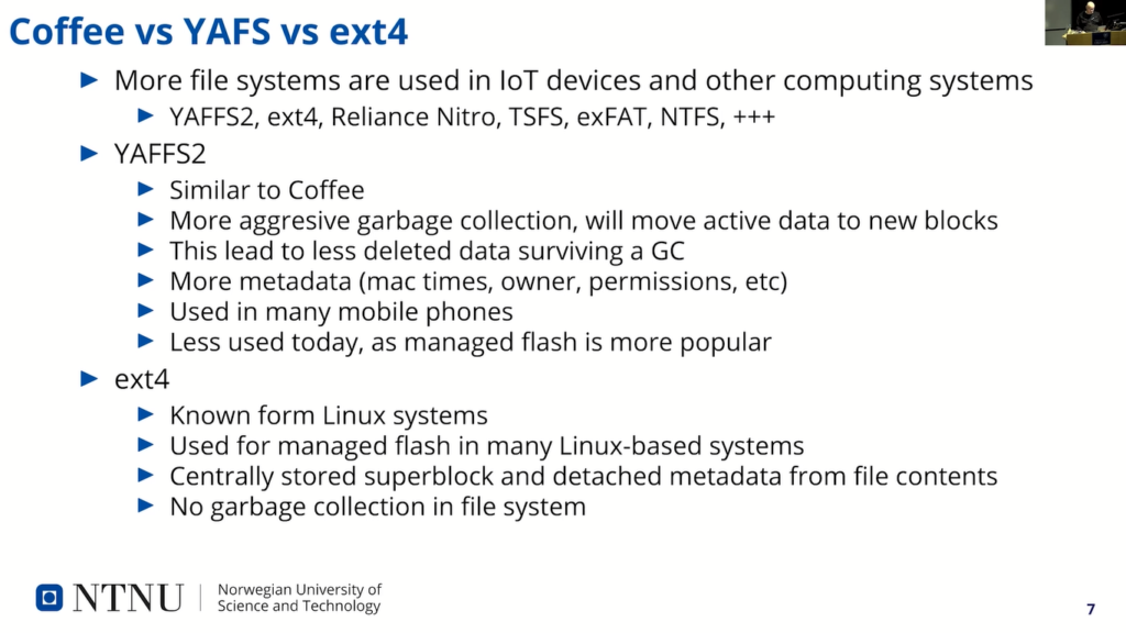
This copying and aggregation of active data from mostly deleted blocks into new blocks means that more of the deleted data will be erased when the collector resets the erased block. The file system also contains more metadata for files. It contains timestamp (when the file was modified, accessed and created), Mac times, owner data, file permissions and so on.
YAFFS2 is used in many places, especially Linux based systems such as Android phones. But the recent popularity, or managed flash, has made the YAFFS file system lose some popularity and ext4 has actually gained the popularity instead in many embedded type of systems.
That system is well known, made for ordinary hard disc, and the flash management system is done in managed flash controller. And the flash controller shows the file system just as a continuous range of address.
So, it’s more centrally placed metadata structure, such as the super block. And I also have the iNotes that contains links to the content data, not, kind of, embedded together with the content data. And of course, ext4 does not do garbage collection by itself, as it assume it can override any written page. (Sorry, I need to get some water.)
And what is volatility? Yeah, volatility is a term that needs to be defined a little bit before we are going to measure it. Most notable use of the word is used in “Order of Volatility”, measures a relative…or it’s a relative measure of how fast data disappears. This term is used in most books on digital forensics.
And we can also think of the volatility terms of the objective lifetime of the data: from the data is created until it’s overwritten (or erased). Another way of thinking of it in terms of the remaining lifetime of the data: time from now (or any point in time actually), until the data is erased.
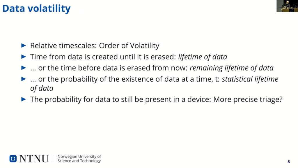
And of course we can also think of it in terms of probabilities, that it’s the probability that data still exist at the time. One of the advantages of being able to better predict the existence data after a time is that the triage can be more precise as we can focus on devices that more likely contains data…is not if you know that data probably already have been overwritten or probably exists still.
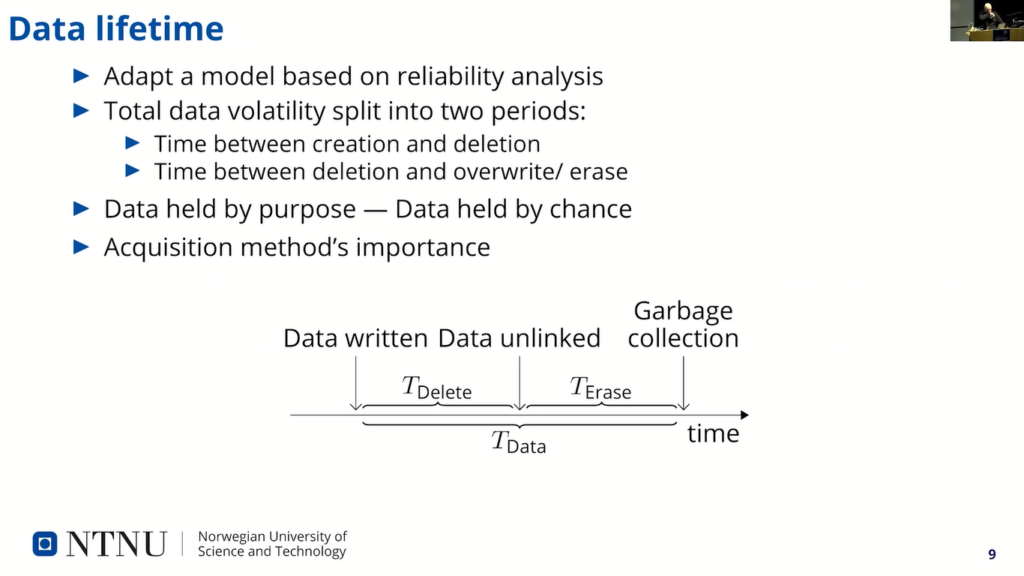
Let’s see. The lifetime of the data can be modeled as the sum of two individual periods of time. The first is the time the data is created on a device to the time it is unlinked or deleted from the file system (so, see the first “TDelete” there). And the next…the second is the period from when data is unlinked until it’s actually overwritten or erased.
So, in many ways we can think of the first period here, TDelete, as the period where the data is held by purpose. The application has a purpose by not deleting the data. And the second period is a period where the data is held by chance, or kind of to the whims or the file system.
First period just depend on the application processing the data, how long it will keep the data alive. And the second is dependent on the system running application, how long it will keep data before it erases it.
And the acquisition method is of course important for which data is available for us. If you use logical acquisition, there is very unlikely that we’ll see any of data that is still exist during the “TErase” phase here, after data is unlinked. And if you use a physical acquisition…we’ll probably see this data that still exist during “TErase”.
(So, just need to cough a little bit. Sorry about that. Got a dry throat now, and speaking.) So, the volatility model we use is itself based on described in our paper towards the generic approach of quantifying evidence, volatility and resource constrained devices from last year, and a reference to that paper can be found in this paper.
This is the high level perspective on the model. The first part of the model here defined as a 6-tuple is that (let’s see, where was I in the manuscript here?) is a storage abstraction layers, or how the different ways data is encoded in abstraction layers.
A couple of examples is that physical storage of the data is as charges on a chip can look quite different from the quasi-physical layer, as read through the flash translation layer. And the data can be readable when read from the operating system, but unreadable when stored encrypted on the physical medium.
The next is the events that affect the system and thereby the volatility. Then we have application activity function. That is how the application handles the data and how fast it will delete it.
And there’s the storage management functions that process the data between the storage abstraction layers, and this can be encryption, flash translation, functions, as we mentioned.
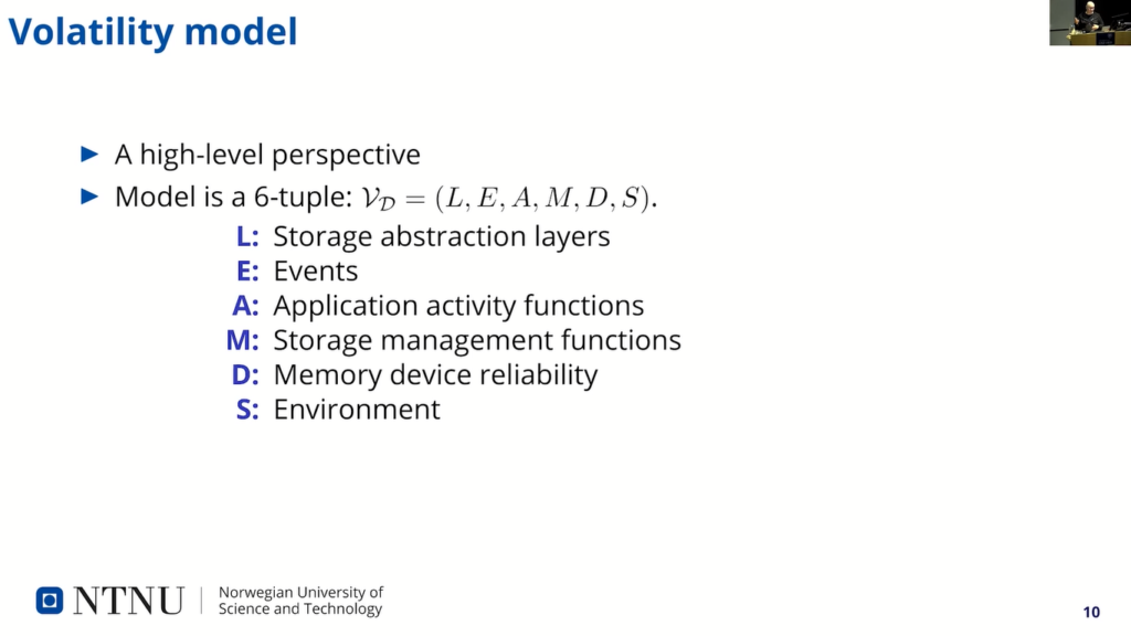
The device reliability gives an upper limit for the reliability, and it’s given us “D” here (or upper limit for lifetime) and it’s given us “D”.
At last, there is the operational environment that can affect the volatility, which is a more statistical nature than the individual events described earlier. We won’t go into details of the whole model here, but rather focus on the storage management functions and how these affect the volatility.
The events and application activity functions are given in experiments and the memory device reliability is not considered in this work, as it’s works on simulated devices and thereby not anything that have physical failures.
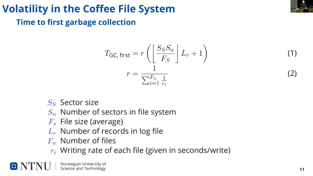
So, we first set out to see the time to first garbage collection. And this is from the start, when we start running the system until the first garbage collection runs. The file system is empty and we start writing files and the time is given by the write rate.
We have first inside the here section SS and SN is the sector size and a number of sectors divided by the, kind of, file file size and the lower number of that plus…times the number of log file entries that are written in order to get the number of writes before default, plus one, because it’s the last one that triggers the garbage collection, and “r” here is the writing rate that is given us the harmonic sum of the individual writing rates.
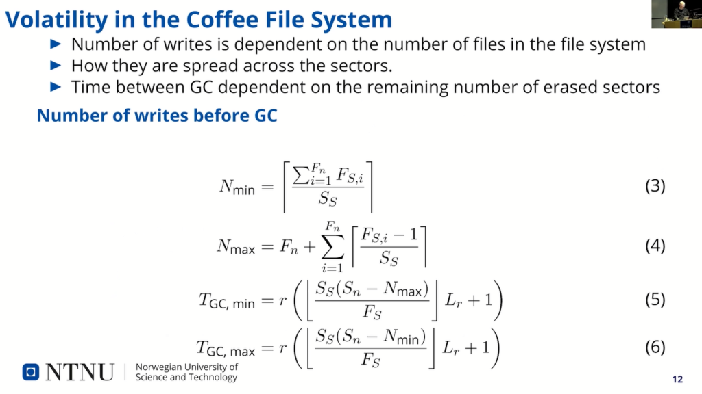
So, that is the, kind of, base model. And number of the writes is dependent on files and their sizes, and the number of sectors on the sector size. Minimum number of remaining sectors are (can be left after a garbage collection) is when all files are packed, and the maximum number of sectors remaining after garbage collection is when each file spans the most number of sectors that will…for a small file, it will span two sectors each file.
This is the…and then you have, kind of, the minimum and maximum time, and that is, kind of, based on this expression… equation I showed on the last slide, but with less sectors.
So, the maximum time a sector can survive is not longer than the longest writing time, or writing rate: when the oldest file is written, the oldest sectors freed up to be garbage collected. Where “TGC” here is the “inter garbage collection time”. And our max is the writing rate of the slowest writing file.
We see that if we count units here, we see that T sector is actually a rate also, but if you take the numerical example here with a file system contain three files that is written on a, kind of, 1 second per write, 50 second per write and 1000 second per write, you see that 256 pages per sect…in each sector, that’s 15 sectors and 22 pages per file and 4 records, we get that it takes about…like, it should take about 635 and 408 seconds between garbage collections and the maximum lifetime should be around 1,270 seconds. (Oh, “=22” there is just a typo from me.)
And of course all this non…like this ceiling and floor functions, make it a little bit difficult to, kind of, give exact results, at least for my mathematics background. And even for simple files system, there’s a need for approximating volatilities.
So, we’ve…last slide, we saw the maximum/minimum times for garbage collection and we don’t really know the number of remaining pages for each run (so our garbage collection run), so we’ll rather hide this uncertainty into a scaling factor that we denote by “K” here. And then we try to measure that by observation instead.
Between the denominator here just is the….assuming a uniform distribution, and it could have been, kind of, put into the scaling factory here. That there needs to be estimated experimentally, but it should be the same for variations of the writing rates.
So, experimental setup. What did we do? The experiments were performed to see how well the theoretical analysts matched the observed results. Contiki devices were set up as standalone devices, and each device had three applications that wrote one file each. We used the Cooja simulator for this, as it comes with the Contiki operating system.
The writing rate of the files were chosen at random from my uniform distribution between 1 second per write up to 1,200 seconds per write, so about 20 minutes between writes. Each simulation run consisted of 16 devices and was run for 10 days. This was repeated 10 times with new writing rates, new devices for every simulation run.
So, in total simulation time for all nodes were 1,600 days, or about 4 years and 4 months simulation time (it runs faster on the simulator though). One of the devices crashed consistently every time and was removed from the analysis.
So, we have…for us to figure out how long the written data existed in memory, we used the Canary tokens. And a Canary token is just a special value that are monitored for access and triggers some response when it is accessed.
So, in our case, the applications running on the devices were writing one token to its file for each writing operation, so I just set a 30 bit number to be written to disc. And we had three applications writing like them, three different tokens, one for each application.
And this made us possible to log both the process…which process that accessed the timestamp, the time and the file system location of the write. The two functions that were patched in operating system is both in the file shown here. The function “program_page” handles the writing on the page and the function “erase_sector” deletes the erase block.
Two parts of the lifetime of the data, as I mentioned earlier, can then be calculated easily: “TDelete”, the first part when a data is active is the time from the token is written in a specific page to the time the token is written next time, because that invalidates the previously written token.
And “TErase” can then be found by subtracting the erase time from the writing time in the same sector (so, when it gets erased, basically), giving us the whole lifetime of the page and that is T data, and if we subtract TDelete, we get TErase. So that’s the kind of how we measured.
So, first we verified that writing rates that we program match to observe values. This was done by calculating the writing rate and compare it with a number of write operations in the log file. And to our surprise, there were about 20% error between expected the observation and (show here in red line) and the observed one.
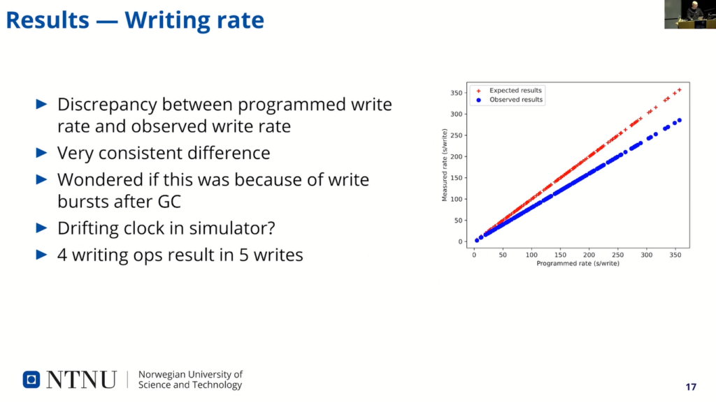
And of course in the paper, I speculate a little bit about why does this discrepancy exist? And while writing these slides, of course, I feel a little bit stupid now. But I thought, or I figured out, that it was of course, because of the function of the file system, that four writes actually triggers five writes on disc.
This extra write is taken into account in a model, so it’s kind of not affecting the results, but it made a little bit headache to understand why this happened, but this should not…doesn’t affect any of the other results.
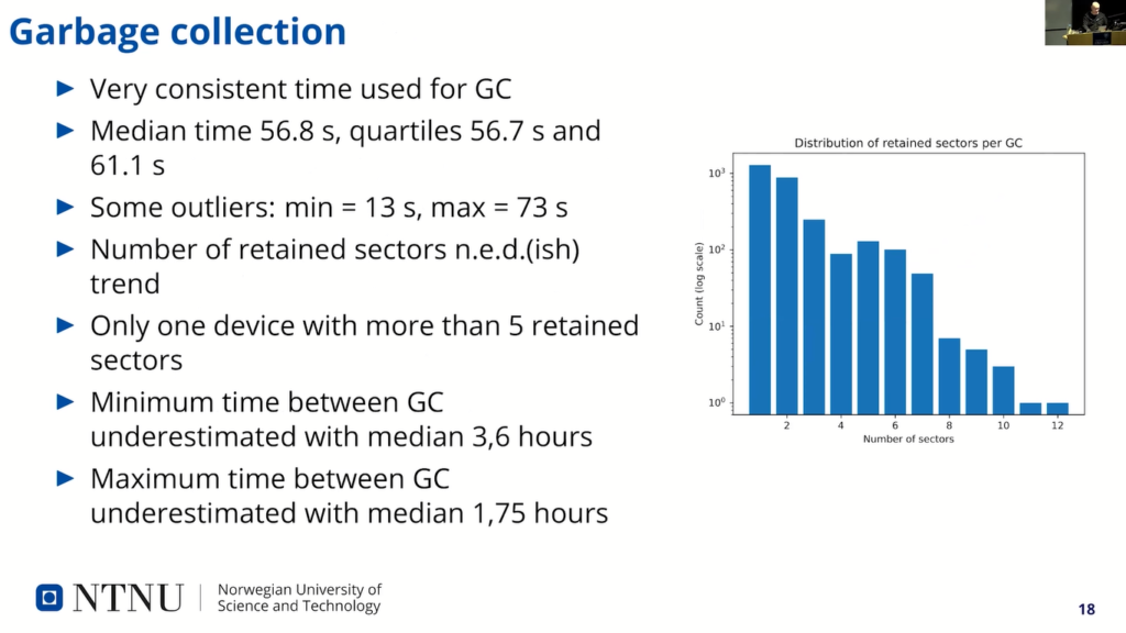
So, garbage collection. Very consistent time used for a garbage collection. It was very stable, around one minute. And some outliers: the minimum time was 13 seconds, maximum was 33. And the number of retained sectors was, kind of, a negative exponential distributed dish trend.
You see that in the table here, where the number of sectors are here and the logarithmic scale of number of garbage collection runs that retained that number of…or deleted that number of…or retained that number of sectors…deleted actually, yeah. Retained, I mean! Retained because it’s one sector retained is most of the time, and it’s quickly decreasing.
So, it was only one device that had more than five retain sectors, much as well with the…that we thought it would be six. But this device had up to 12 retain sectors, and we saw that the one that…where the garbage collection only lasted 30 second also matched the one where they retained 12 sectors, so it’s very few sectors that were garbage collection there.
Minimum time between garbage collections were underestimated with a median about 3.6 hours and maximum time was also underestimated. So, it was clearly some discrepancy in the analytical model.
Average lifetime (I see, I start to be finished soon since I see something moving here!)…average retention time for all pages were about 7 hours, and that is for a system that had maximum writing rate of 20 minutes per write. And the maximum time was about five hours, no five days and eight hours…nine hours.
And the table here shows the result when I applied the scaling factor to the approximation. It’s not too bad…point to half an hour of, like, half an hour wrong for the most wrong device. And also the distribution of lifetime of the pages for all pages for all devices combined is shown here, and with a logarithmic scale on the vertical scale.
So, last analysis was distribution of the lifetime. So, we just tried to see if there was any matching distribution that could explain the data. It kind of…so this is from two individual devices: the upper one is a typical one, the one we saw most of…and the gray area here shows that the first is, like, calculative time to the garbage collection, between 0 and TGC.
And the second gray area was where I just tried to figure where…or I divided the time between garbage collection on the number of sectors and placed this (the gray area) on the third last one, and then it matches quite well. And except for the lower here, where it’s the…you see the two gray areas there also, but they’re squished into the left corner there, so this one was very atypical and also contained the data for a very long time. This was one that contained that for five days.
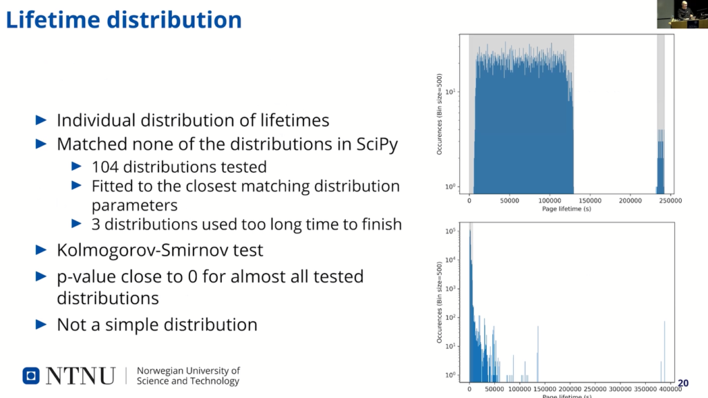
We used the Kolmogorov-Smirnov test to test the various distribution, but none really fits anything, so it’s not a simple distribution at least.
The thing we didn’t do was to look at other file systems, also this methods, kind of like, we wanted to make something that was really easy to do for the, like, forensic investigator going out, trying to figure out where this…where the data might be.
But of course this model is not simple enough for…to be used yet, at least. And maybe we need to generalize, maybe figure out a way to generalize this. So, we did analytically estimate the volatility, and we found a method for measuring the volatility for devices running Contiki OS, the same can probably be done with the other operating systems. And yeah, in the end we saw there were many special cases the analysis didn’t take into account.
So, that was everything for me!
Bruce: Good. Thanks a lot, Jens-Petter. So, in the interest…ah, let’s give him a hand. Thanks. So, in the interest of time, I think we’ll take one question quickly from the audience and one from the online. So, any questions in the audience fast? First hand, I see. No? How about in the chat? How are we looking?
Moderator: We don’t have any questions in the chat. I have a question.
Bruce: Okay.
Moderator: Sorry, this is a running theme now! I was wondering if you could just for my understanding help to bridge the conceptual gap a little bit between a sort of concrete understanding of data volatility in these IoT systems, and then how this can be used, sort of, at a higher level, at a forensic level for evidence in cases and things.
Jens-Petter: Yeah. Well, the idea is that this can be one of the tools for deciding which system to, kind of, investigate further. Like, in case you have, like, maybe come to the scene of a crime, it’s might be thousands of devices around an area, which one you have limited the number of resources available for doing this investigation, and you need to find which device…or you don’t have time or resources to, kind of, acquire like everything: go to the cloud provider, figure out who that this; fog systems, figure out where those are; the individual nodes, figure out where those are and get the data out.
So by…at least have an estimation of how fast the data disappears from those devices, it’s also easier to come for example, say, “okay, I want to use…take…collect evidence from this device first because the data will disappear more quickly from this one than from that one.”
Or you can say, “okay, this one has been laying around so long, so it’s probably…it’s far over its probable lifetime of data, so I don’t really need to look into that one. I will focus on this one that more probably contained the evidence I’m looking for.” So that was kind of the background for this.
Moderator: Great. Thank you.
Bruce: Okay. Thanks.