Determining the previous locations a suspect or victim visited, and the roads traveled, is one of the main questions investigators use vehicle data to answer. When tracklogs, navigation points or other geo-tagged data is recovered, this is a pretty straightforward task. What happens when a vehicle does not record any of these? Can the question, “Where has this vehicle been?” still be answered?
Recently, in a missing persons case out of New Jersey, investigators were faced with this exact scenario. The recovered vehicle did not record any geolocation data. Despite this, investigators used other time-stamped, distance-based data to identify key areas of interest with a technique called reachability analysis. This ultimately led to the recovery of the victim’s body.
In this article, we are going to show you how to drive your investigations forward with non-geotagged vehicle data, reachability analysis and a few open-source tools to identify previous locations and areas of interest when traditional geolocation data is not an option.
To demonstrate how reachability analysis works, we asked our research team to drive a route from Berla Headquarters (HQ) to a local Park and Ride, simulating a vehicle being abandoned after a crime. The team chose a 2017 Jeep Grand Cherokee with a Uconnect system for this task. Uconnect systems sometimes record tracklogs, but not consistently. Since this is one of our research vehicles, the team already knew we would not get any geolocation data when we acquired the system data.
What the Uconnect system does provide, like many other vehicle systems, is reliable odometer events with timestamps. This allows us to determine both the distance traveled and the time it took. We acquired the data on-site at the Park and Ride and then returned to HQ to analyze it.
Establish Knowns
The process of identifying previous locations or areas of interest, starts with building a timeline of the vehicle’s movements. To do this, we will establish the knowns and identify the unknowns.
What we know is that the vehicle was driven between two known locations — Berla HQ as the starting point and the local ‘Park and Ride’ as the endpoint. What we don’t know is if the vehicle made any stops along the way. If it did, where did those stops occur?
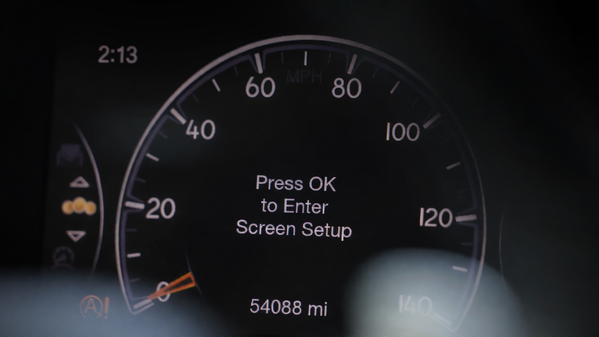
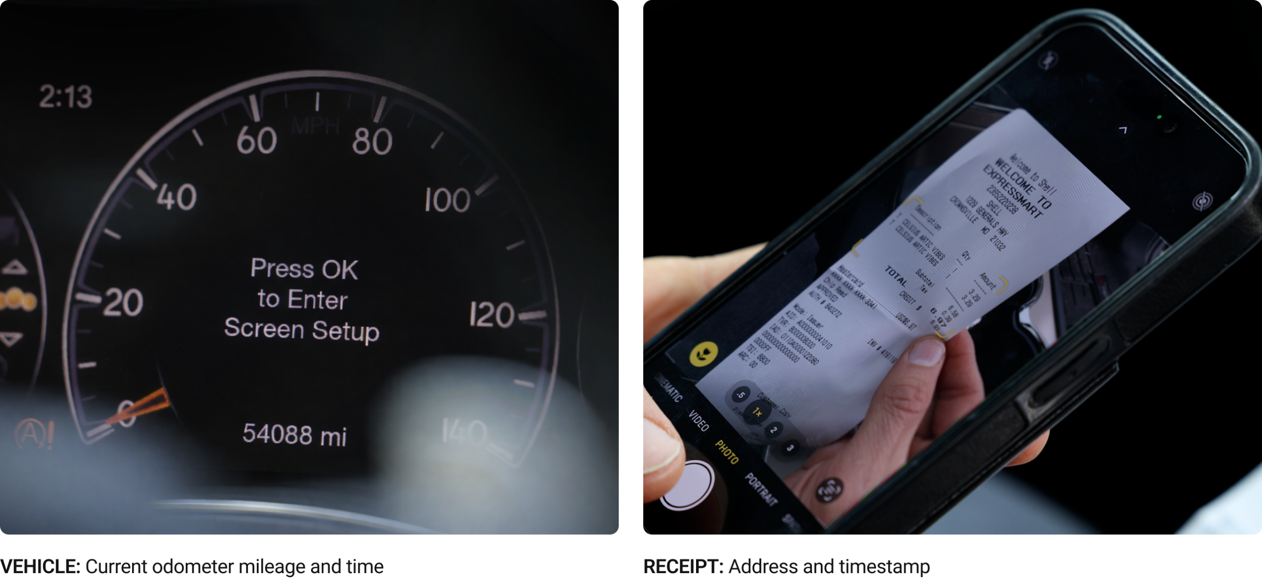
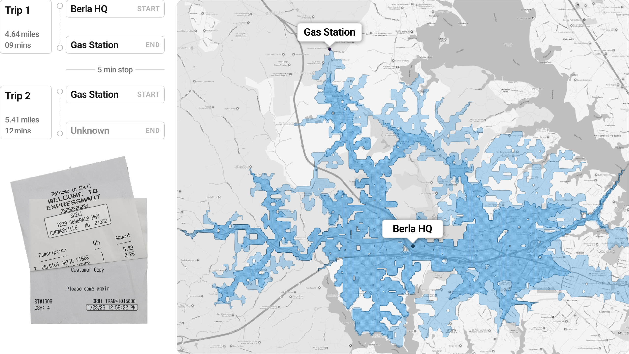
We know the current odometer reading is 54088 miles; we noted it when we got into the vehicle at the Park and Ride to do the acquisition. We also found a receipt for a local gas station, conveniently left in the cup holder.
Using the odometer reading we recorded at the Park and Ride, and the data we acquired from the vehicle, we know the vehicle arrived at the Park and Ride at 1:29:23 pm. Working backwards, we can see the vehicle left Berla HQ at 12:45:42 pm. The odometer events show that approximately 14 miles were traveled over a 43-minute period.
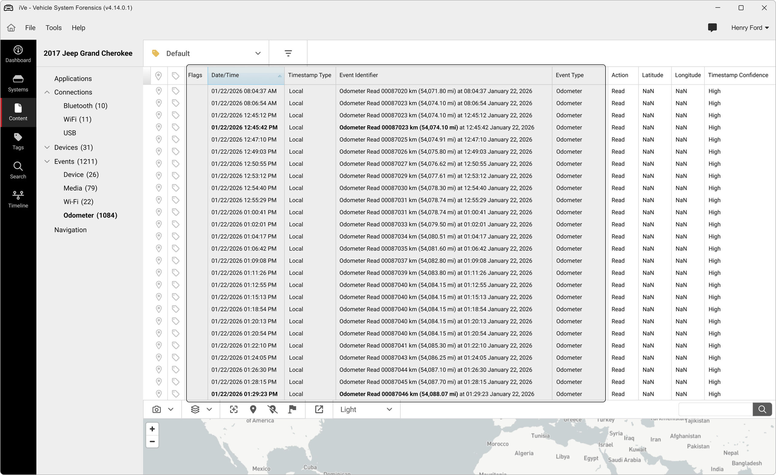
Having driven the route, we know the actual trip is approximately 6.1 miles and takes about 12 minutes. This clearly indicates that the vehicle did not take the optimal path and must have deviated from the main route during its journey.
Identify Unknowns
To identify unknown locations where stops were made, we will analyze the odometer events to determine whether the overall journey can be broken into independent trips. For each trip, we need to identify the start and stop location, distance traveled, and the time it took.
We are looking for patterns or a break in a pattern in the odometer events. We will focus on the timestamp of each event and the odometer reading. Consecutive events with increasing timestamps and increasing odometer values mean that the vehicle is on the move. Gaps in time between two events where the timestamp difference is greater than one minute and the odometer value does not change, indicate the vehicle stopped at a location and the engine was shut off. Consecutive events where the odometer value does not change and timestamps increase over several minutes indicate the vehicle was stopped at a location for a prolonged period with the engine running.
Using these patterns, we are able to determine that the overall journey, starting from Berla HQ and ending at the Park and Ride, consists of three distinct trips with two unknown stops.
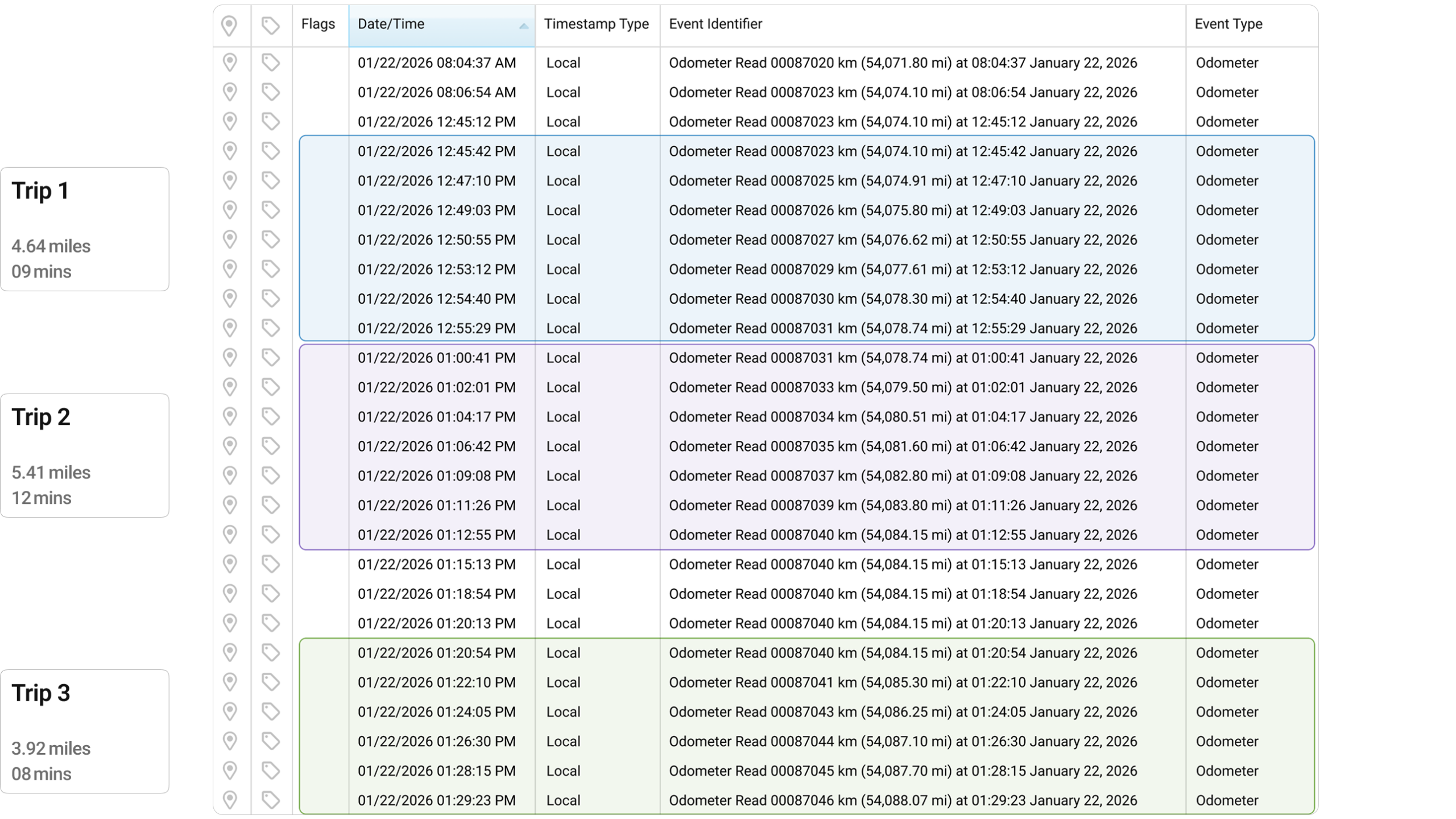
Between Trip 1 and Trip 2, we see a five-minute gap between events. No odometer events were logged during this time. This indicates the vehicle made a stop and the engine was turned off. Between Trip 2 and Trip 3, we see odometer events being logged for 8 minutes with timestamps increasing while the odometer values do not change. This indicates the vehicle stopped with the engine running.
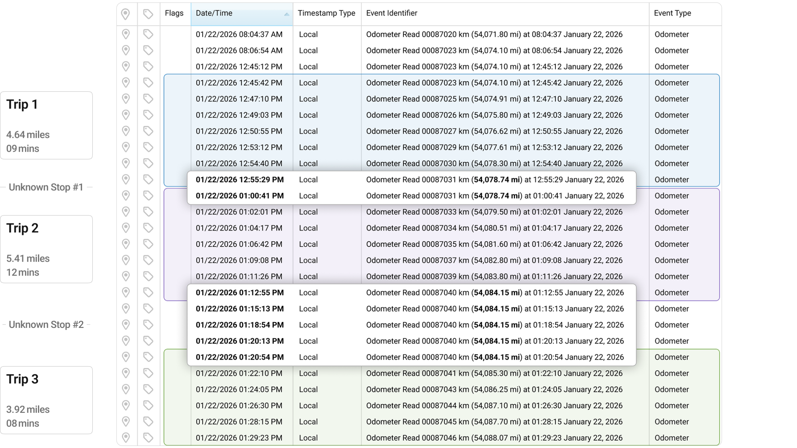
With these trips identified, we are ready to build our timeline, starting with our known locations. We will enter the distance and time from each trip into the reachability tools to help us determine possible or plausible locations for the unknown stops.
Reachability Analysis
Reachability tools are used to answer questions like, “Where can this vehicle get to in 10 minutes?” or, “How far can this vehicle get in 10 miles?” They require a start location and either a time value or distance value. What you get back is a time-isochrone or distance-isochrone overlaid on a map. An isochrone is a map-based way to show how far you can travel within a given amount of time or distance from a location, using the actual road network, not a straight-line. It represents all possible routes, collapsed into a boundary.
Standard reachability tools, like Valhalla , do not work for our purpose; they force us to choose time or distance. We can get around this by running two separate queries via Valhalla’s APIs , and combining the resulting time-isochrone and distance-isochrone for each trip in a geospatial visualization tool, like QGIS .
We’ll begin with Trip 1 since it has a known start location. We’ll mark Berla HQ on the map and then import Trip 1’s time-isochrone (dark blue) and distance-isochrone (light blue). This gives us all possible endpoints for Trip 1.
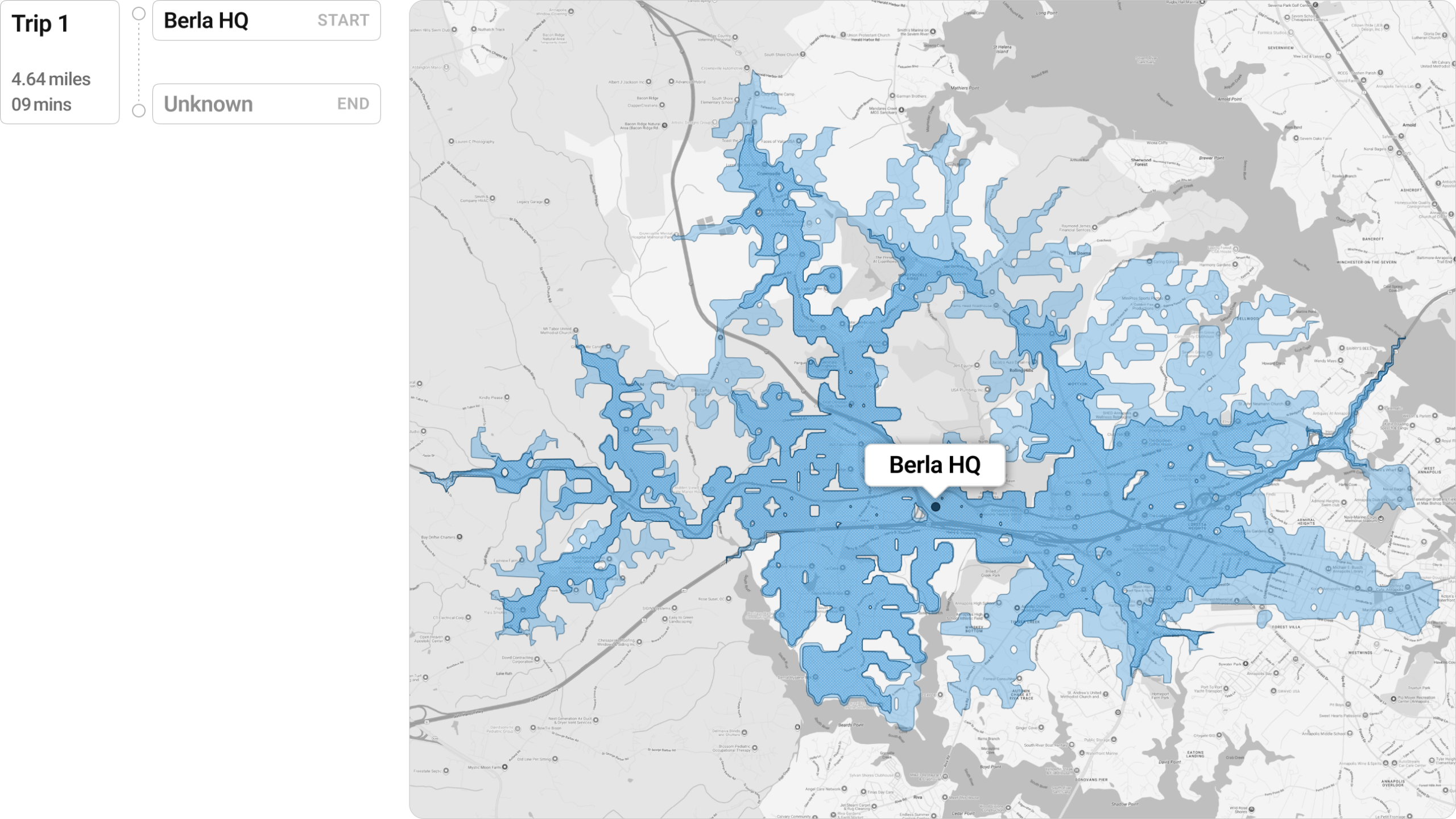
The receipt we found for the local gas station, conveniently left in the cupholder of the vehicle, has a timestamp of 12:59:22 PM. That timestamp is within the time period of Stop 1. Using this address we will mark the gas station on the map. When we do that, we see it falls nicely within the distance-isochrone (light blue), which is the outer boundary of Trip 1. Taking this and the timestamp of the receipt into account, we can conclude that the gas station is the end location of Trip 1, which makes it the previously unknown location of Stop 1.
We will use the Gas Station as the known start location for Trip 2 and import Trip 2’s time-isochrone (dark purple) and distance-isochrone (light purple). This will give us all the possible endpoints for Trip 2. We’ll mark the Park and Ride on the map since it is the known end location for Trip 3.
Because Trip 3 only has a known ending location, we need to generate reverse-isochones and work backward from the known endpoint. Reverse-isochrones use the same math as normal isochrone, but the edges of the boundaries are reversed. By asking Valhalla to give us reverse-isochones, we are asking it to answer the question, “From where could this vehicle have arrived?” This is a simple, but important, distinction that gives us more accurate boundaries.
We’ll import Trip 3’s reverse-time-isochrone (light green) and the reverse-distance-isochrone (dark green). This will give us all the possible starting locations for Trip 3.
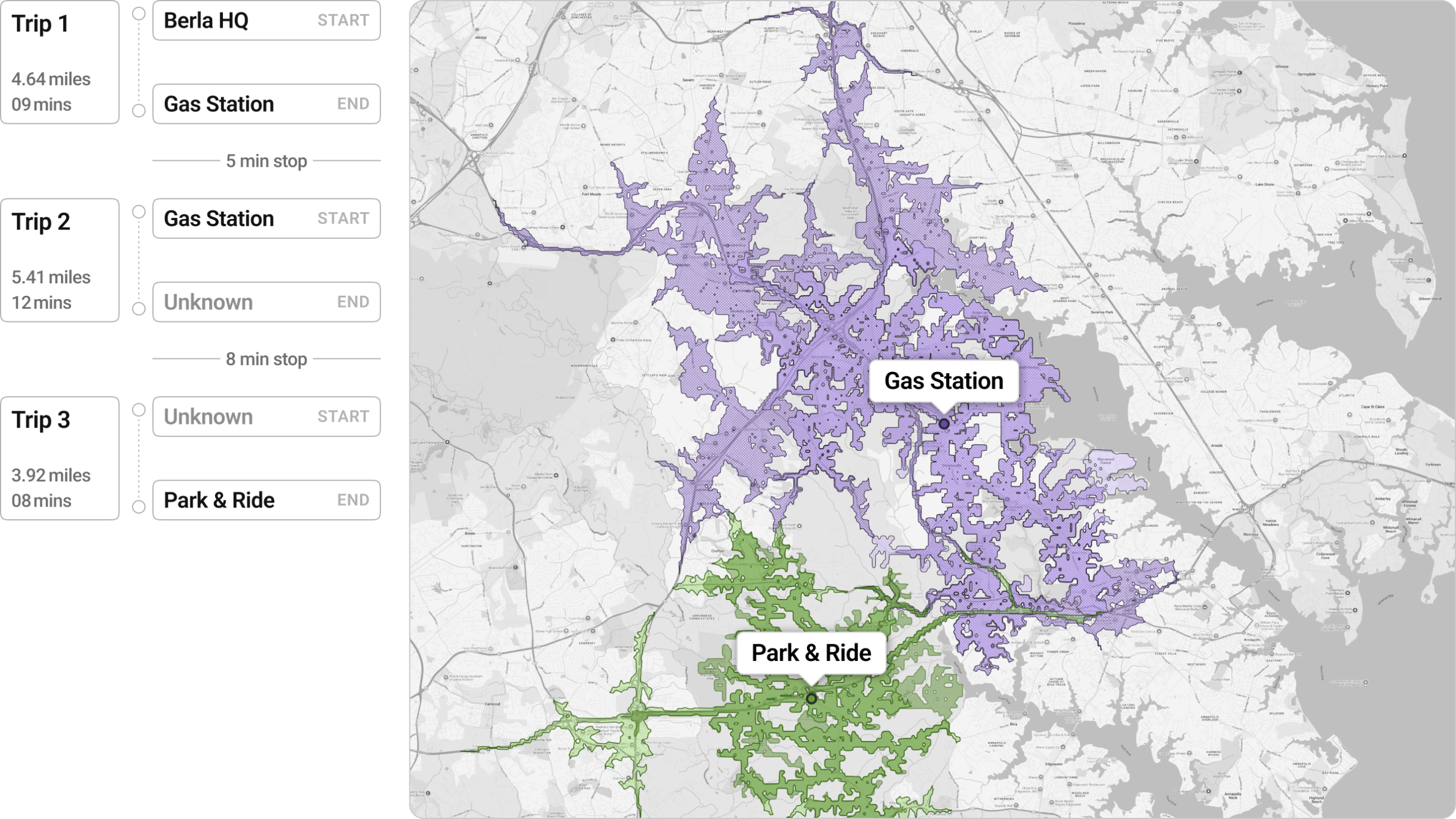
With Trip 2’s time-isochrone and distance-isochrone, as well as Trip 3’s reverse-time-isochrone and reverse-distance-isochrone on the map, we will process the isochrone with the Intersection Geoprocessing Tool in QGIS. The results identify the intersecting locations of the time isochrones and distance isochrones of Trip 2 and Trip 3. The intersecting areas identify all of the possible locations of unknown Stop 2.
The intersection of the time isochrones (brown) gives us four large areas of interest. The intersection of the distance isochrones (red outline) gives us a single 135 yard stretch of road to investigate.
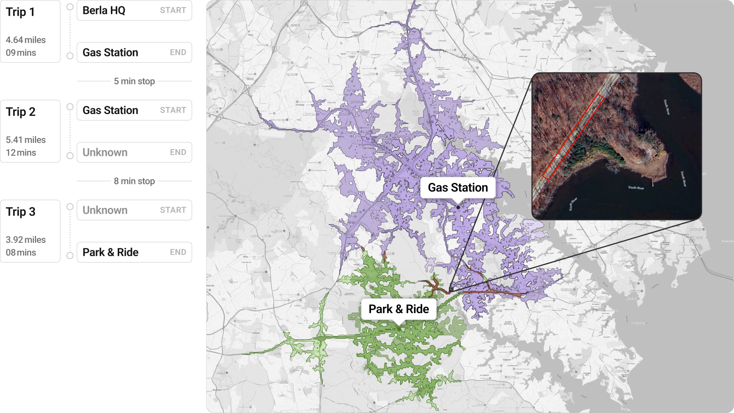
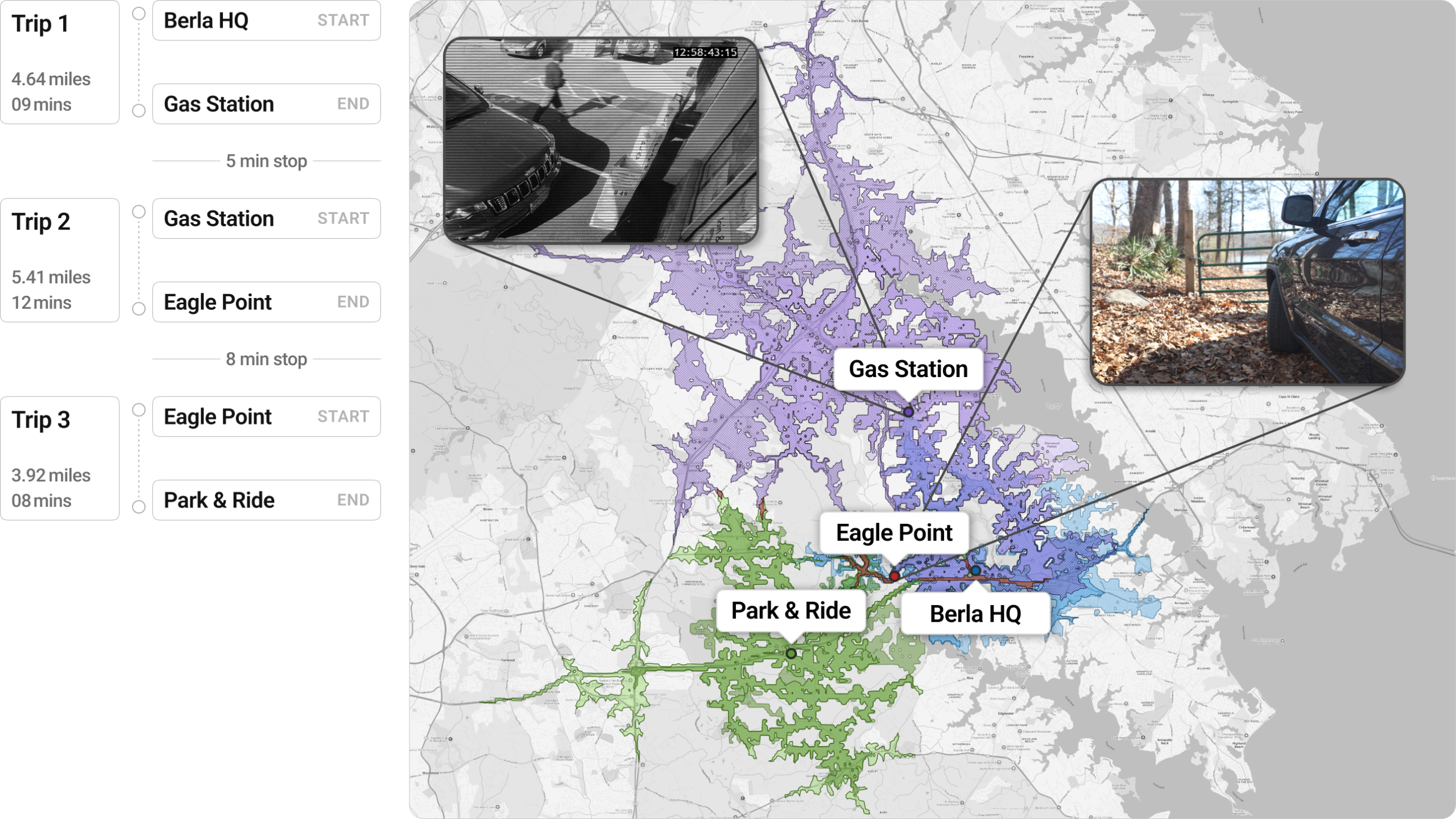
Based on the optimal route from the Gas Station to the Park and Ride, we are going to surmise that the end location for Trip 2 and the start location of Trip 3 occurred along a 135 yard stretch of road near Eagle Point. When we reviewed our findings with the Research Team, they validated the location of Stop 1 was the Gas Station and the location of Stop 2 was at the roadside gate of Eagle Point .
Conclusion
By analyzing odometer events and combining the results with open-source tools to perform reachability analysis, investigators can identify unknown locations even without traditional geolocation data. These techniques drive investigations forward by converting vehicle data into defensible, location-based intelligence. This validates or eliminates leads and uncovers key evidence faster. Ultimately, this provides closure to victims and their families, ensuring justice prevails when it matters most.