Speed Against The Backlog: What’s Slowing You Down And How To Fix It

Over 25,000 devices. Waiting. This figure comes from the UK policing inspectorate, HMICFRS, and does not capture everything that is likely already in the pipeline. Behind each device is a case. Behind each case is a person waiting for answers. At the heart of the issue is a fundamental question: how quickly can data be extracted from a device? How can you improve the imaging performance? Because until you have the image, nothing else can be started.

It’s not a simple answer. As one DFIR practitioner put it:

“Imaging speed is so variable, based on the content of the drive, the output speed, the tool used … It’s easier not to think about it.“

Easier, but not an option when the backlog is this size. There are a lot of variables and pitfalls – and not all of them are within your control. For example, a damaged evidence drive will slow things down unpredictably. But not every drive is damaged. This article focuses on the factors that are within your control.

The Slowest Link Sets the Speed 

There’s one rule that never changes: imaging speed is always limited by the slowest device in the session. If the source reads at 100 MB/s and the target writes at 500 MB/s, the imaging speed will still be 100 MB/s. The ceiling is always the floor of the slowest drive.

But the weakest link isn’t always the drive. A worn-out cable, a network shared by multiple examiners all running high-performance tasks simultaneously – any of these can become the bottleneck. The rule is simple. The variables behind it are not.

Drive Type Matters

A DFIR professional described it well:

“Imaging an old 500GB external HDD right now. Over SATA it got 35% done before it failed. Now trying again over 2.0 and it’s got 16 hours left. Then the SSD I’m imaging on the other computer is going 175 MB/s and will be done in less than 15 minutes. Amazing the contrast”.

Keep in mind that a healthy HDD is slower than a healthy SSD.

What you can do:

1. Use a modern, high-speed drive as your storage for images (like NVMe SSDs or enterprise-level SAS drives). You can check the write speed of different models on websites such as UserBenchmark. 
2. Always diagnose your drives. Don’t just focus on evidence drives. For Source drives it helps to get a realistic estimation of imaging time and shows whether data is accessible, helping you decide which drive deserves your attention first. On target drives, Diagnostic detects degradation early. If you are an Atola imager user, simply click the ‘Diagnostic’ button in the interface. If you are not, check tools like CrystalDiskInfo and Hard Disk Sentinel.
3. Gain an understanding of SMART values. Reading them before imaging begins takes minutes and can completely transform your approach. Some attributes point to physical wear, such as reallocated sectors, uncorrectable errors and spin retry counts. On HDDs, for example, this can indicate magnetic layer degradation. On SSDs, they can indicate worn NAND memory. Other attributes tell a different story. Total LBAs Written, for example, is not just a wear indicator — it is also a forensic data point. A sudden spike in write activity before seizure may indicate a large-scale file transfer or deliberate data movement.

A Novel About Cables

“In a digital forensics lab, we agonise over CPU choice, write blocker brands, and software licences that cost more than a small car (or house in some cases). Then we plug all of it into a £3 cable from a drawer and wonder why the extraction is taking long enough to finish a novel”.

That quote comes from a DFIR field. It’s also, quietly, one of the most accurate descriptions of how imaging speed gets lost in practice. High-end hardware running through a degraded cable doesn’t run at high-end speeds. It runs at cable speeds. And cables don’t announce when they’ve become the bottleneck.

What you can do:

1. Test before you trust. USB-C cables can be particularly deceptive. While the sleeve may say ‘USB 3.2 Gen 2’, the silicon inside may tell a very different story. An eMarker reader can verify the cable’s declared capabilities, but only a real transfer test can confirm its actual speed and stability. Check both before deployment.
2. Inspect regularly and replace early. Network cables degrade over time. Connectors loosen. A cable that worked fine six months ago may now be silently dropping packets, reducing throughput without triggering any obvious errors. Include cable inspection in your lab maintenance schedule – don’t wait for slow extraction speeds to indicate a problem.
3. Skip the enclosure when you can. External drive enclosures add a translation layer between the drive and your imager – and that layer has its quirks and failures. Where the investigation allows, remove the drive and connect it directly. Fewer intermediaries means fewer variables, and fewer variables means faster, cleaner results.

None of this is very exciting. But in a system where 25,000 devices are waiting to be examined, every hour matters.

Imaging Settings: Small Decisions, Real Consequences

Default settings are optimized for speed. Don’t change them without a reason. But when you have one, here’s what matters:

1. Enable reverse imaging for degraded drives. Reading from the end first can get more data before the drive deteriorates further.  The trade-off: drive cache is disabled, so overall speed drops. Use it when the drive calls for it.
2. Calculate one hash. Running MD5 and SHA1 simultaneously adds overhead that’s easy to avoid. When policy allows and speed matters, one hash is enough. Also take into consideration that SHA-1 & MD5 are faster than SHA-256 & SHA-512.
3. Don’t overlook your output format. Raw is the fastest. If you need a container, AFF4 is generally quicker than E01 – and better optimized for compression. That said, compression only helps when it can actually reduce the data size. If the source is encrypted, or full of videos, images, or archives, entropy is too high for compression to gain anything. In those cases, skip it.

Network Setup: When Peak Hour Really Counts

“We used to work to the server but network issues meant we had to do it locally.”

It’s a common story for forensic labs. Network imaging is the goal – but infrastructure problems push investigators back to local workflows, adding steps and adding time. When imaging over a network, the infrastructure between source and destination matters just as much as the drives themselves.

What you can do:

1. Configure your network for high throughput. Start with the basics: use faster interfaces – 10GbE minimum, 25GbE where possible. If you’re imaging to a Samba server, set min receivefile size = 16384 to reduce overhead on large transfers. And enable Jumbo Frames (MTU = 9000) across all network devices. It reduces the number of packets needed to transfer large files and can noticeably improve throughput on a well-configured network.
2. Keep the network path short. Every additional node between your imager and the server adds latency. Minimize hops, and make sure every node in the chain supports 10 Gigabit connections or more.
3. Check your cables. As covered earlier, degraded cables rarely announce themselves – they just slow everything down. The same applies to your network infrastructure. CAT 6 is the minimum for a 10GbE network, and network cables deserve the same routine inspection as everything else in your lab.
4. Consider who else is on the network and when. A lab where multiple examiners are simultaneously imaging to a server is a lab where everyone’s throughput is shared. Peak hours matter. The question came up directly in a DFIR community discussion:

“Do all forces make a second copy immediately or do they wait until the network is quieter, the evening perhaps?”

“We were told it needed to be as soon as possible to get the second copy secure.”

“I would imagine it is done when the network is quiet – all automated, of course.”

Or a practical middle ground:  

“A network connection certainly won’t ever be as fast as working locally on a SSD.  Moving data in the evenings and weekends kept me from clogging the network with all that traffic”.

There’s no universal answer. But the fact that DFIR practitioners are actively debating when to run imaging jobs around network load says a lot about the real constraint.

5. And don’t overlook the hardware itself. If a router or switch is running at sustained CPU or memory usage above 80%, it becomes a bottleneck regardless of what’s connected to it. Check device utilization periodically.

Server Setup: the End of the Line Matters Too

“We work direct to servers. However we have recently experienced issues with seeing 0 byte media files when generating reports.”

The network path matters – but so does what’s waiting at the end of it.  A well-configured network connected to a poorly set up server will still create a bottleneck.

What you can do:

1. Configure RAID server properly (preferably use NVMe or SAS drives). A single drive or JBOD setup limits throughput by design. RAID 5, 6, or 10 will give you better speed and redundancy.
2. Choose the right file system. File systems that support sparse files speed up writes. Those with built-in copy-on-write features slow them down.
3. Monitor drive health. Slow or degraded server drives limit imaging speed just as a slow source drive would. The same tools mentioned earlier apply here – CrystalDiskInfo and Hard Disk Sentinel give you a clear picture of what’s happening before a failing drive becomes a bigger problem.
4. Review user quotas. Bandwidth limits on individual accounts can quietly throttle imaging jobs without any obvious error. Make sure high-priority tasks have the resources they actually need.

Image More, Automate the Rest

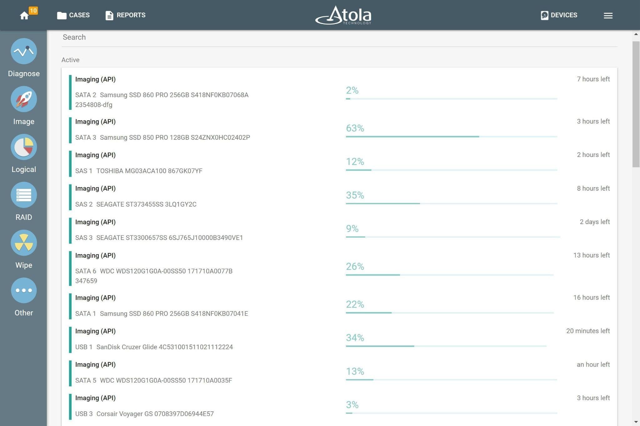
Cables, settings, server configuration, network load – all of it matters. But even a perfectly optimised single imaging session is still just that: a single session. When 25,000 devices are waiting, the question shifts from  “how fast?” to “how many simultaneously?” That’s where the architecture of your imager becomes the deciding factor. Atola TaskForce 2 was built around exactly these two constraints – parallel processes and automation.  Automation takes it further. Via Web API, external software can launch, track, and stop imaging sessions programmatically – no manual handoffs, no waiting between cases. The moment imaging ends, analysis can begin.

What You Can Do With Atola Taskforce 2

• Image 25+ drives simultaneously at 25 TB per hour
• Automatically reassemble and image RAIDs
• Acquire data even from damaged drives
• Integrate drive imaging into your workflow via Web API
• Get the full power of the server-grade hardware and two 10Gb network ports (upgradeable to 25Gb)

The backlog is a systemic problem. No single device solves it. But the right hardware – running in parallel, integrated into an automated workflow – means fewer hours lost to variables you can control.

May the speed be with you!