
The Forensic Aspects of Analysis of Deepfake Videos Based on AI Algorithms
Zeno Geradts: Good morning. I would like to present Forensic Aspects of deepfakes. So this is a short presentation of five minutes and I will shortly go through it. Nowadays, it’s quite easy to make a deepfake. So you can download DeepFaceLab which is freely available on the internet and make your own deepfake, or if you don’t have the computational power you can also use Google Colab to make those deepfakes yourself. So they will combine two faces in one version, and then you can speak with another voice and pretend to be another person.
So there are many examples available, many are also with presidents and you can find many of those examples on the internet. And one of the issues is that [indecipherable] people might say, “No, it was not me. It was a deepfake.” And then you have to examine if a deepfake was made.
We see also that it’s quite easy to make audio deepfake. With only five minutes of training there it’s already possible to make a rather good deepfake audio, some voice cloning. So it’s been known for four years that this is possible. One of the issues there is, of course, we need to also to use the same [indecipherable] as the normal person would use. So this is something to consider when making a good audio deepfake.

There are many best practices in the world on finding deepfakes. I will not go into detail on all those parts, but you will find best practice guide for image authentication SWGIT [indecipherable]. You can do a detailed, of course, metadata, but that’s easy to spoof with the mixed photo response on uniformity, so that’s a kind of fingerprint of the sensor that might work. You can try to detect the image creation, or some kind of staging and some continuity issues.
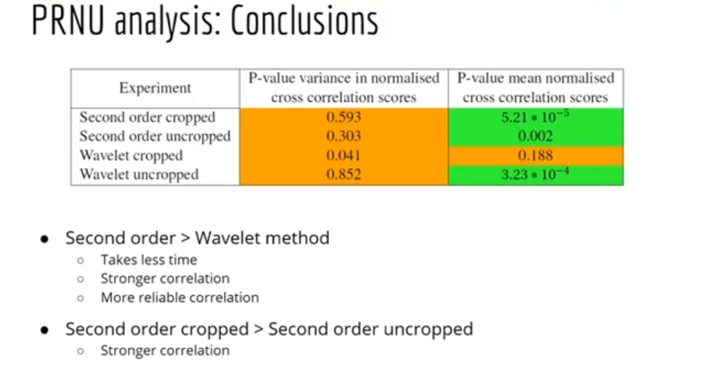
If we look into a PRNU analysis, we did this in the past and in the past it worked quite well. So, using the fingerprint. If you don’t have the camera, it does not work that well anymore. So unfortunately, this method is working less than one year ago. So we see that the algorithms for making deepfakes are getting better.
So the newest detection methods, at least which were new a few months ago, they are often image-based. So that’s something we see that could be also a better way of detecting it by making it video-based, so based on the compression schemes, et cetera, that are used.
So, video-based as I said, there you can also use this compression and also the loss that has been generated. And the compression is an issue with detection, because this is often used when uploading images to YouTube or social media and makes it more complicated to detect those deepfakes.
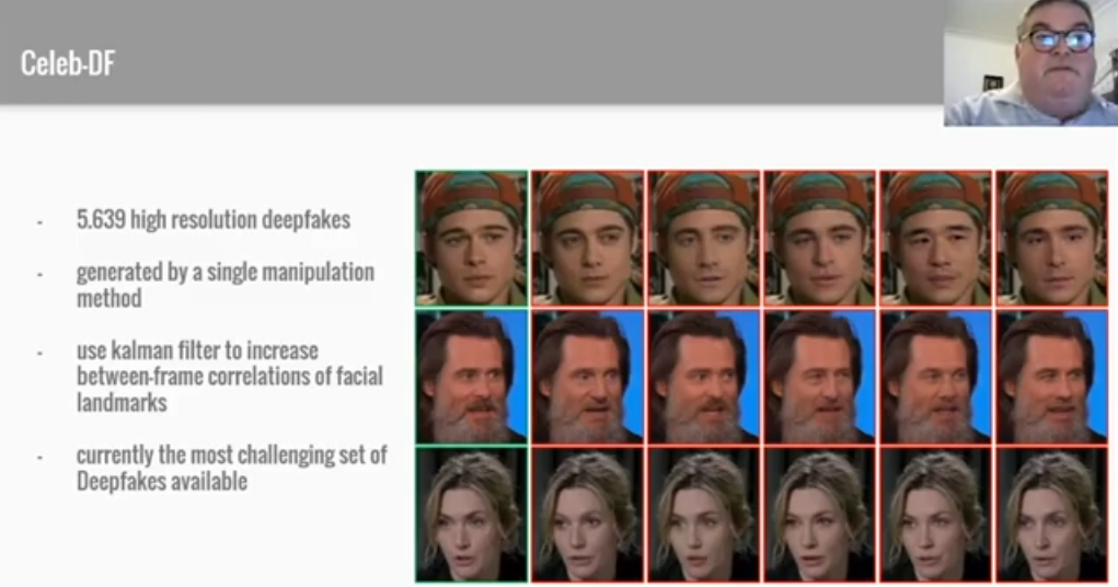
There are many databases for celebrity deepfakes you might download from the internet. This is one of the most challenging sets of deepfakes that we saw. Deepfake Detection Challenge is less real and of course it’s best to have real-world data because that’s the kind of data that we also will receive in real cases.
So there are several models and we’ll not go into detail on all the models, but nowadays we see that EfficientNet-B7 works quite well according to the literature and it’s available pre-trained on ImageNet. And then we see also in the challenges that this performs best, at least that they have an accuracy of around 84%.
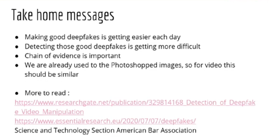
So the take home messages I would like to give is making good deepfakes is getting easier each day. Detecting those good deepfakes is getting more difficult. The chain of evidence is important. And of course, in the past, we are also used to Photoshopped images. So for video, this should be similar, and we also have several publications that you might want to read about this topic.
I would like to thank you very much for your attention, and if you have any questions, I would be happy to address them. So you can send me an email on this. Okay, thank you very much.
Feature Extraction of Protest Demonstration on Lihkg Discussion Forum
Ao Shen: Hi, everyone. This is Ao Shen from the University of Hong Kong. This research is by Dr. K.P. Chow and me, and our title is Feature Extraction of Protest Demonstration on Lihkg Discussion Forum.
Here is the agenda of this presentation. We will first overview the Lihkg dataset, then talk about the motivation of this research. Then it is the experiment on multilabel classification. Finally, we’ll have a conclusion and talk about the future of work.
In today’s cyberspace, many cyber crimes leave traces in social media platforms, such as Facebook and online discussion forums, and potential criminal activities may be posted on social media. In this way, the online platforms are the places for detecting potential crimes and obtaining traces.
The Lihkg discussion forum is a well-known multi-category discussion forum in Hong Kong. Some activity organizers will post notification messages in advance and their supporters or regular users can intermittently read, participate, and post their comments.
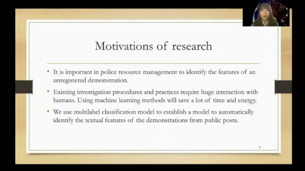
From August 2019, most of the discussions on the forum refers to public gatherings and demonstrations. The demonstrations in Hong Kong over these past months have astonished the world, but whether a particular activity constitutes a criminal offense depends on the local laws and regulations. But it is still important in police resource management to identify the features of an unregistered demonstration. So this study established a model to automatically identify the features of the demonstrations from public posts.
We divided our experiment into four parts: data collection and labeling, post vectorization, multi label classification model, and finally is the experiment result. The first step is data collection. We collect the posts and the Lihkg Current Affairs section from 2019 August to October. Most of the posts are in Traditional Chinese or Cantonese. And the sentence in this bracket is the English translation for this presentation.
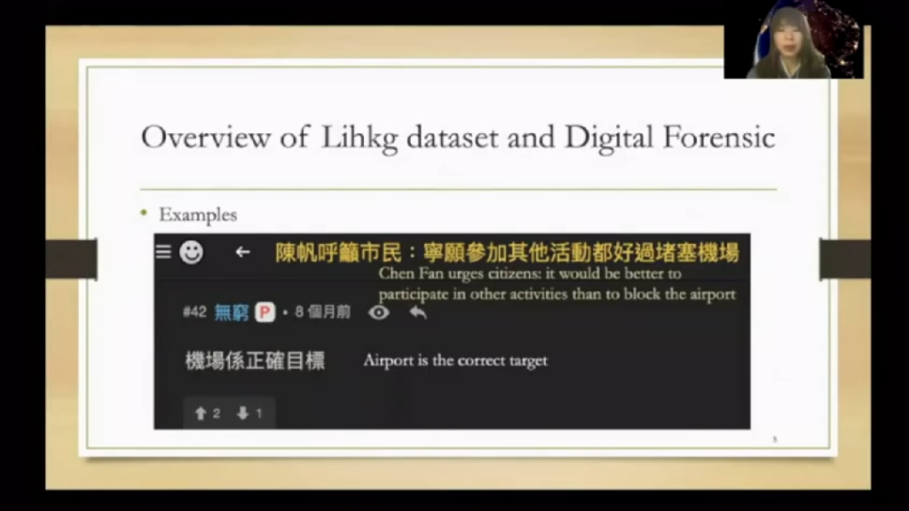
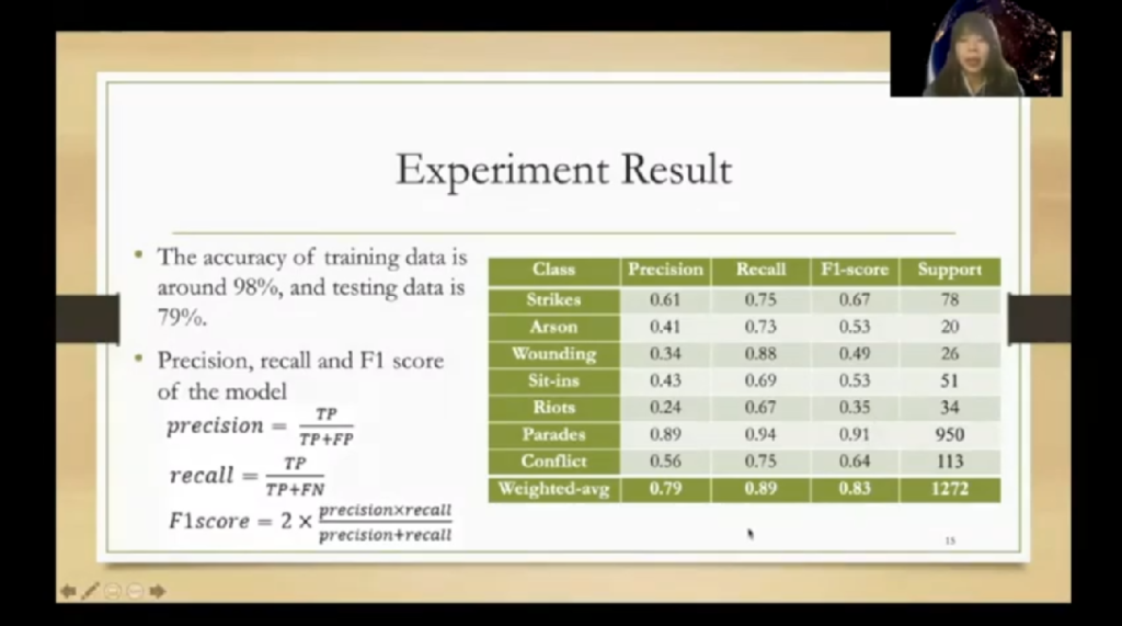
About data labeling, in total there are seven labels: strikes, arson, wounding, sit-ins, parades, rails and conflict. And we randomly select 1,272 posts to label the data like this, like the table shown here.
The second part is the post vectorization. We first used a Doc2Vec to transfer the textual post to vector metrics, and then used the Pearson correlation coefficient to calculate the coefficient matrix, to find the relationship between the post and the seven labels. And then this metrics is the input of the multilabel classification model.
For the classification model, we use MLP neural network to build the model. It is a class of the feedforward artificial neural network. And I show the structure and the information of the model here. The accuracy, precision, recall, and F1 score as shown in this slide. And from the weighted average value here, we can see that MLP has a good performance and reliable classifying to the corresponding labels. I think the label data is unbalanced. It’s still difficult to identify some minority features.
We can also output some high correlation topics, up here in each class. So based on these topics, it is feasible to describe the subject and understand the urgency of the corresponding demonstration. To make a conclusion, the Floyd demo demonstration will not only disrupt business and traffic, but also affect social security and threaten the social order.
We use MLP multilabel classification methods to understand the specific forms and characteristics of the harmful demonstrations on online forums so that it can provide the theoretical support and applications and posts to assign resources and have a proper monitoring of the activity schedule.
The future research will attempt to study the relationship between the subjects and discourses on a deeper level. That’s the end of this presentation, thank you for listening.
The Calibration of Step Count Logs in Apple Health Data
Luke Jennings: The Calibration of Step Count Logs in Apple Health Data. We compared the Apple Health database step count logs with the acceleration and rotation characteristics, which constituted a robust step identification to create a controlled step test rig, to adjust metrics such as lag, bias and aggregation through three distinct experiments, which consist of different step intensities and durations.
The results from experiments one and two are overlapped, showing the lag present in the step count logs. Likewise, experiments two and three overlap showing the bias present in the step count logs. Experiment three highlights the aggregation of step count error.
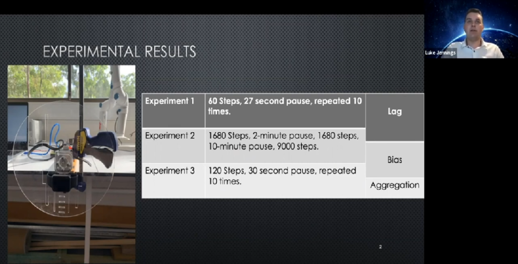
The first experiment consisted of the rig performing 60 steps, pausing for 17 seconds and repeating 10 times. The first observation here is that Apple Health records these as 58 steps. In MATLAB, we superimposed the Apple Health logs in blue over the axivity accelerometer measurements in red.
Here the step interval initiates at 32.0 seconds, while the watch logs the step interval 7.0 seconds later. Allowing for time synchronization differences or ±1.0 seconds for the axivity data and ±0.5 seconds for the Apple Health log data, we apply a combined error of ±1.12 seconds to determine a measured time lag of between 5.9 and 8.1 seconds on this first sample.
The last step concludes at 63.7 seconds with the Apple Health log stopping at 65 seconds. This is a time lag of 1.3 ±1.1 seconds. Importantly, the acceleration interval, including attack and decay, is 31.7 seconds, but the Apple Watch reports a bias interval of 26 seconds.
This table shows the variation in lag times across the 10 intervals, referenced to an experiment time log initiated 39 seconds before the first Apple Health interval log. Note that we start to see the start lag get smaller over time and the end lag get negative. This might be a sample period bias or some sort of clock shift. We need to review carefully in future experiments when we want to calibrate our log to millisecond accuracy.
The sharp attack or rising edge of each sawtooth in this figure represents the start lag while steps accumulate before the step interval start time is logged. The shortened step log interval compresses the step rate. So then once the interval starts, steps are counted at a faster rate than excitation, effectively catching up and reducing the count bias. We see a compressed time interval catching up with ground truth.
In the second experiment, we ran the apparatus for 150 minutes in four long intervals: three of 14 minutes with 1,680 steps each; and one of 75 minutes, which is about 9,000 steps. The purpose here is to see how long intervals behave.
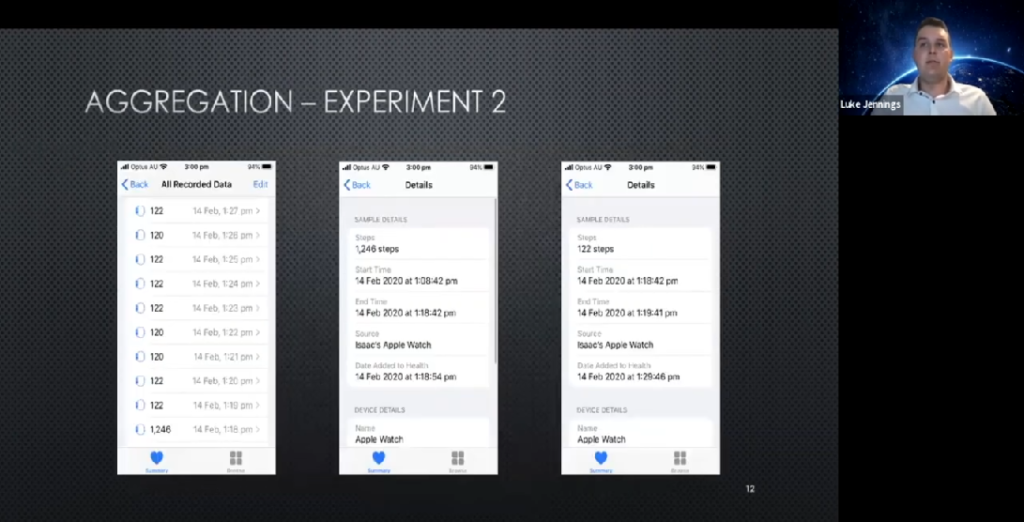
It can be seen that the error in this step count does not show a clear positive or negative bias. There are spikes at the beginning of each time interval, but eventually it catches up. If the short-term transient bias caused by the lag between initial step excitation and the logging initiation is excluded, it could be seen that the cumulative error in this experiment lies between +13 or -8 steps over a total of 14,040 steps, or a cumulative error of 0.1%.
We see a relatively high error for any given interval, but over the day, it looks like it balances out. Here, for experiment 3, we see many step intervals not terminating correctly in Apple Health, unlike the previous cases where it aggregates many step periods into singular, larger periods.
Of particular interest here is that the first measurement interval shows 708 steps, capturing a total of 720 steps over a 510-second interval. Although the instantaneous step rate is 2.0 steps per minute, the inclusion of the five 30-second rest periods means that the reported average step right over 507 seconds is actually 1.4 steps per second.
There are many limitations for our preliminary results. For example, we attempted to reduce the delay between consecutive step intervals as low as possible until the Apple Watch could not differentiate the gap and write different step periods as a single log. Multiple testing suggests this is around 15 steps or around 7.5 to 8 seconds of activity at our current settings. However, repeating this experiment did not always reproduce the same result. Some of the experiments stopped being able to differentiate the intervals, even with a two-minute break in between. Thank you for listening to my presentation.